Page 267 - Distributed model predictive control for plant-wide systems

Hot-Rolled Strip Laminar Cooling Process with Distributed Predictive Control 241

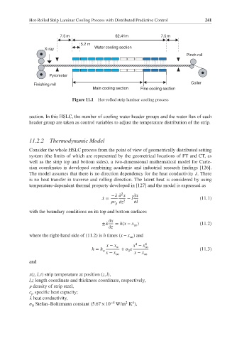
7.5 m 62.41m 7.5 m
5.2 m
Water cooling section
X-ray
Pinch roll

Pyrometer
Finishing mill Coiler
Main cooling section Fine cooling section

Figure 11.1 Hot-rolled strip laminar cooling process

section. In this HSLC, the number of cooling water header groups and the water flux of each
header group are taken as control variables to adjust the temperature distribution of the strip.

11.2.2 Thermodynamic Model

Consider the whole HSLC process from the point of view of geometrically distributed setting
system (the limits of which are represented by the geometrical locations of FT and CT, as
well as the strip top and bottom sides), a two-dimensional mathematical model for Carte-
sian coordinates is developed combining academic and industrial research findings [126].
The model assumes that there is no direction dependency for the heat conductivity . There
is no heat transfer in traverse and rolling direction. The latent heat is considered by using
temperature-dependent thermal property developed in [127] and the model is expressed as

2
− x x
̇ x = − l ̇ (11.1)
c z 2 l
p
with the boundary conditions on its top and bottom surfaces
x
± = h(x − x ) (11.2)
∞
z
where the right-hand side of (11.2) is h times (x − x ) and
∞
4
x − x w x − x 4 ∞
h = h + (11.3)
w 0
x − x x − x
∞ ∞
and
x(z, l, t) strip temperature at position (z, l),
l,z length coordinate and thickness coordinate, respectively,
density of strip steel,
c specific heat capacity;
p
heat conductivity,
4
2
Stefan–Boltzmann constant (5.67 × 10 −8 W/m K ),
0