Page 271 - Distributed model predictive control for plant-wide systems

Hot-Rolled Strip Laminar Cooling Process with Distributed Predictive Control 245

1 2 3 … n s Strip thickness
∆z
… …
∆l
… l s−1 l s … l n−1 l N
l 1
l 0
z
Subsystem i Subsystem N
l
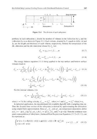
Figure 11.4 The division of each subsystem

problem. In each subsystem s, denote the number of volumes in the l-direction by n and the
s
z-direction by m as shown in Figure 11.4. Each volume, denoted by V, equals to ΔlΔz. Δl and
Δz are the length and thickness of each volume, respectively. Denote the temperature of the
s
ith z-direction and the jth l-direction volume by x .Let
i,j
x 0 = x , i = 1, 2, … , m (11.7)
FT
i,n s
x N = x N , i = 1, 2, … , m (11.8)
i,n s i,n s −1
The energy balance equation (11.1) being applied to the top surface and bottom surface
volumes leads to
s ( ( s ))
1, j 1 h 1, j ( ) 1
̇ x s =− x s − x s −Δz x s − x − v(x s − x s ) (11.9)
1, j s s 2 2, j 1, j s 1, j ∞ 1, j 1, j−1
cp Δz Δl
1, j 1, j 1, j
s ( ( s ))
m, j 1 h m, j ( )
̇ x s =− x s − x s −Δz x s − x
m, j s s 2 m−1, j m, j s m, j ∞
cp Δz
m, j m, j m, j
1 s s
− v(x − x ) (11.10)
Δl m, j m, j−1
For the internal volumes, it is
s
1 i, j s s s 1 s s
s
̇ x =− (x − 2x + x )− v(x − x ) (11.11)
i, j 2 s s i+1, j i, j i−1, j i, j i, j−1
Δz cp Δl
i, j i, j
̇
where v = l is the coiling velocity, x s = x s−1 when j = 1 and x s = x s+1 when j = n .
s
i, j−1 i,n s−1 i, j+1 i,1
In industrial application, the measurements are available digitally with a sampling time Δt.
Thus the discrete-time version of the subsystem is derived by approximating the derivatives
s
s
s
using simple Euler approximation. Since , , and cp are temperature-dependent, define
i, j i, j i, j
s
s
s
2 s
s
s
s
a(x )=−Δt ∕(Δz cp ), (x )=Δta ∕ and =Δtv/Δl. Then the nonlinear state
i, j i, j i, j i, j i, j i, j i, j
space representation of subsystem s, deduced from the previous Equations (11.7)–(11.11), can
be expressed as
{
s
s
s
s
s
x (k + 1) = f(x (k)) ⋅ x (k)+ g(x (k)) ⋅ u (k)+ D ⋅ x s−1 (k)
n s−1 s = 1, 2, … , N (11.12)
s
s
y (k)= C ⋅ x (k)