Page 276 - Distributed model predictive control for plant-wide systems

250 Distributed Model Predictive Control for Plant-Wide Systems

However, the local optimal control decision of its downstream neighbors and the future
optimal states of its upstream neighbors are not available to subsystem s, and hence the esti-
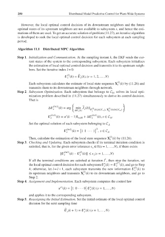
mations of them are used. To get an accurate solution of problem (11.27), an iterative algorithm
is developed to seek the local optimal control decision for each subsystem at each sampling
period.

Algorithm 11.1 Distributed MPC Algorithm

Step 1. Initialization and Communication. At the sampling instant k, the EKF sends the cur-
rent states of the system to the corresponding subsystem. Each subsystem initializes
the estimation of local optimal control decision and transmits it to its upstream neigh-
bors. Set the iterative index l = 0:
(l)
̂
U (k)= U (k), (s = 1, 2, … , N)
s
s
(l)
Each subsystem calculates the estimate of local state sequence X (k) by (11.26) and
s
transmits them to its downstream neighbors through network.
Step 2. Subsystem Optimization. Each subsystem that belongs to C solves its local opti-
W
mization problem described in (11.27) simultaneously to derive its control decision.
That is
{ }
ΔU (l+1) (k)= arg
s min J (k)| (l) (l)
s
U (k)(j∈N −i ), X (k)(h∈N +i )
ΔU s (k) j h
(l+1) s (l+1)
U s (k)= u (k − 1)I 1×M +ΔU s (k), s ∈ C W
Set the optimal solution of each subsystem belonging to C
A
T
[
]
U (l+1) (k)= 11 ··· 1 , s ∈ C
s A
(l)
Then, calculate the estimation of the local state sequence X (k) by (11.26).
s
Step 3. Checking and Updating. Each subsystem checks if its terminal iteration condition is
satisfied, that is, for the given error tolerance ∈ ℝ(s = 1, … , N), if there exists
s
(l+1) (l)
‖U s (k)− U (k)‖ ≤ (s = 1, … , N)
s
s
*
If all the terminal conditions are satisfied at iteration l , then stop the iteration, set
∗
∗
the local optimal control decision for each subsystem U (k)= U (l ) (k), and go to Step
s s
(l)
4; otherwise, let l = l + 1, each subsystem transmits the new information U (k) to
s
(l)
its upstream neighbors and transmits X (k) to its downstream neighbors, and go to
s
Step 2.
Step 4. Assignment and Implementation. Each subsystem computes the control law
[
]
s∗
∗
u (k)= 10 ··· 0 U (k)(s = 1, … , N)
s
and applies it to the corresponding subsystem.
Step 5. Reassigning the Initial Estimation. Set the initial estimate of the local optimal control
decision for the next sampling time
∗
̂
U (k + 1)= U (k)(s = 1, … , N)
s s