Page 277 - Distributed model predictive control for plant-wide systems

Hot-Rolled Strip Laminar Cooling Process with Distributed Predictive Control 251

Step 6. Receding Horizon. Move horizon to the next sampling time, that is, k + 1 → k,goto
Step 1, and repeat the above steps.

The online optimization of HSLC, which is a large-scale nonlinear system, is converted
into several small-scale systems via distributed computation; thus computational complexity
is significantly reduced. In addition, information exchange among neighboring subsystems
in a distributed structure via communication can improve control performance. Through this
method, the whole temperature evolution of the strip is controlled online, which provides pos-
sibilities of producing many new types of steel with high quality (e.g., the multiphase steel).
To prove the validation of the proposed strategy, both numerical simulations and experiments
on a HSLC experimental apparatus are implemented in the next section.

11.4 Numerical Experiment
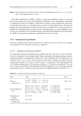
To test the validation of the proposed method, low-carbon C2 type steel is taken as an example.
The parameters of C2 strip steel are shown in Table 11.1.

11.4.1 Validation of Designed Model

An experiment on full-scale industrial plant is performed with a strip of 3.51 mm in thickness
to test the validation of the designed model. In the experiment, the spatial meshing chosen to
validate the model is composed of 5 volumes of 0.7 mm in thickness and 30 volumes of 2.7 m
in length, that is, m = 5, n = 30. The water fluxes in the main cooling section and in the fine
3
2
2
3
cooling section equal to 150 m /(s m ) and 75 m /(m s), respectively. The resulting prediction
of CT and the measurement of CT are shown in Figure 11.5. The curve of predictive CT is very
close to that of measurement. The phenomenon that the predictive curve is smoother than the
measurement curve is caused by the second term in the right-hand side of the model (11.1).
Table 11.1 Thermal and physical properties of the strip

Item Value Units
{ ( ( )) s
56.43 − 0.0363 − c v − v × x
Thermal 0 s 0,j Wm − 1 K − 1
s 56.43 −(0.0363 − c(v − v )) × x m,i
0
conductivity
i,j
⎧ s s
8.65 + (5.0 − 8.65) (x − 400)∕250, x ∈[400, 650)
⎪ i,j i,j
s s
⎪ 5.0 +(2.75 − 5.0)(x − 650)∕50, x ∈[650, 700)
− 6
2
Thermal diffusivity i,j i,j × 10 m s − 1
s
s
⎨ 2.75 +(5.25 − 2.75)(x − 700)∕100, x ∈[700, 800)
s
a(x ) ⎪ i,j i,j
i,j s s
⎪5.25 + 0.00225(x − 800), x ∈[800, 1000]
i,j i,j
⎩
Temperature of 25 + 273.5 K
ambient
Temperature of 25 + 273.5 K
cooling water