Page 274 - Distributed model predictive control for plant-wide systems

248 Distributed Model Predictive Control for Plant-Wide Systems

11.3.4 Local MPC Formulation

As for subsystem s ∈ C , the strip temperature is controlled by a local MPC. The local MPC
W
is formulated based on neighborhood optimization and successive linearization of prediction
model. The details of it are presented next.
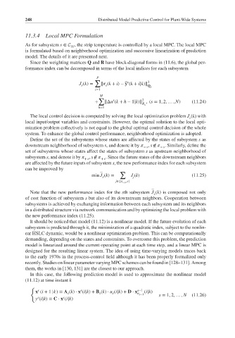
Since the weighting matrices Q and R have block-diagonal forms in (11.6), the global per-
formance index can be decomposed in terms of the local indices for each subsystem

P
∑ s 2
J (k)= ‖r (k + i)− ̂ y (k + i|k)‖
s
s
Q s
i=1
M
∑ s 2
+ ‖Δu (k + h − 1|k)‖ , (s = 1, 2, … , N) (11.24)
R s
h=1
The local control decision is computed by solving the local optimization problem J (k) with
s
local input/output variables and constraints. However, the optimal solution to the local opti-
mization problem collectively is not equal to the global optimal control decision of the whole
system. To enhance the global control performance, neighborhood optimization is adopted.
Define the set of the subsystems whose states are affected by the states of subsystem s as
downstream neighborhood of subsystem s, and denote it by , s ∉ . Similarly, define the
− s − s
set of subsystems whose states affect the states of subsystem s as upstream neighborhood of
subsystem s, and denote it by , s ∉ . Since the future states of the downstream neighbors
+ s + s
are affected by the future inputs of subsystem s, the new performance index for each subsystem
can be improved by
∑
min J (k)= J (k) (11.25)
s j
j∈{ −s ,s}
Note that the new performance index for the sth subsystem J (k) is composed not only
s
of cost function of subsystem s but also of its downstream neighbors. Cooperation between
subsystems is achieved by exchanging information between each subsystem and its neighbors
in a distributed structure via network communication and by optimizing the local problem with
the new performance index (11.25).
It should be noticed that model (11.12) is a nonlinear model. If the future evolution of each
subsystem is predicted through it, the minimization of a quadratic index, subject to the nonlin-
ear HSLC dynamic, would be a nonlinear optimization problem. This can be computationally
demanding, depending on the states and constraints. To overcome this problem, the prediction
model is linearized around the current operating point at each time step, and a linear MPC is
designed for the resulting linear system. The idea of using time-varying models traces back
to the early 1970s in the process-control field although it has been properly formalized only
recently. Studies on linear parameter varying MPC schemes can be found in [128–131]. Among
them, the works in [130, 131] are the closest to our approach.
In this case, the following prediction model is used to approximate the nonlinear model
(11.12) at time instant k
{
s
s
x (i + 1 |k) = A (k) ⋅ x (i|k)+ B (k) ⋅ u (i|k)+ D ⋅ x s−1 (i|k)
s s s n s−1 s = 1, 2, … , N (11.26)
s
s
y (i|k)= C ⋅ x (i|k)