Page 272 - Distributed model predictive control for plant-wide systems

246 Distributed Model Predictive Control for Plant-Wide Systems

where
[ ( ) T ] T
s
s T
s
x = x s (x ) ··· (x ) T ;
1 2 n s
[ ] T
s
x = x s x s ··· x s , (j = 1, 2, … , n ) (11.13)
j 1,j 2,j m,j s
s
is the state vector of subsystem s, y is the average temperature of the last column volumes of
s
subsystem s, u is the input of subsystem s and is defined as follows:
{ ( ) b
c
s
u = 2186.7 × 10 −6 × ⋅ v∕v 0 ×(F ∕F ) , s ∈ C W
0
s
s (11.14)
u = 1, s ∈ C
A
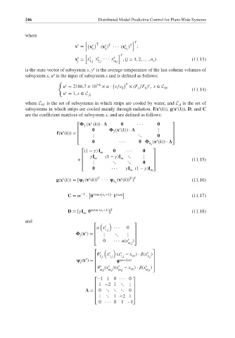
where C is the set of subsystems in which strips are cooled by water, and C is the set of
W A
s
s
subsystems in which strips are cooled mainly through radiation. f(x (k)), g(x (k)), D, and C
are the coefficient matrices of subsystem s, and are defined as follows:
⎡ (x (k)) ⋅ ··· ⎤
s
1
s
2
s
f(x (k)) = ⎢ (x (k)) ⋅ ⋮ ⎥
⎢ ⋮ ⋱ ⎥
⎢ s ⎥
⎣ ··· (x (k)) ⋅ ⎦
n s
⎡(1 − ) I m ··· ⎤
⎢ I m (1 − )I m ⋱ ⋮ ⎥
+ (11.15)
⎢ ⋮ ⋱ ⋱ ⎥
⎢ ⎥
⎣ ··· I m (1 − )I ⎦
m
s
T
T T
s
s
g(x (k)) = [ (x (k)) ··· (x (k)) ] (11.16)
1
n s
[
C = m −1 ⋅ 1×m⋅(n s −1) 1×m ] (11.17)
D = [ I m m×m⋅(n s −1) T (11.18)
]
and
( )
a x 1,j ··· 0
⎡ s ⎤
s
(x )= ⎢ ⎢ ⋮ ⋱ ⋮ ⎥
j
⎥
0 ··· a(x )
⎢ s ⎥
⎣ m,j ⎦
( )
⎡ s x s (x s − x ) ⋅ (x )
s ⎤

⎢ 1,j 1,j 1,j ∞ 1,j ⎥
s
(x )= (m−2)×1
j ⎢ ⎥
⎢ s s s − x ) ⋅ (x ) ⎥
s
(x )(x
⎣ m,j m,j m,j ∞ m,j ⎦
−11 0 ··· 0
⎡ ⎤
⎢ 1 −21 ⋱⋮ ⎥
= ⎢ 0 ⋱⋱⋱ 0 ⎥
⎢ ⎥
⋮⋱ 1 −21
⎢ ⎥
⎣ 0 ··· 01 −1⎦