Page 268 - Distributed model predictive control for plant-wide systems

242 Distributed Model Predictive Control for Plant-Wide Systems

emission coefficient ((x/1000)[0.125x/1000 − 0.38] + 1.1),
x ambient temperature, and
∞
h convection heat transfer coefficient (W/mm 2 ◦ C) on the surface of strip.
w
The radiation boundary condition is only applicable out of the water-cooling section. The
transfer coefficient h is only applicable in the water-cooling section and is calculated as fol-
w
lows:
( ) ( ) ( ) c
a
b
2186.7 x v F
h = 6 (11.4)
w
10 x 0 v 0 F 0
◦
2
3
where x = 1000 C, v = 20 m/s, F = 350 m /(m min), a = 1.62, b =− 0.4, c = 1.41, v is the
0 0 0
velocity of strip, and F is the flux of cooling water.
11.2.3 Problem Statement
The technical targets of HSLC refer to CT and the temperature drop curve of strip caused by
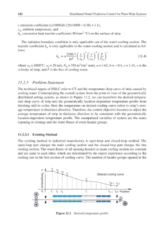
cooling water. Contemplating the overall system from the point of view of the geometrically
distributed setting system, as shown in Figure 11.2, we can transform the desired tempera-
ture drop curve of strip into the geometrically location-dependent temperature profile from
finishing mill to coiler. Here the temperature on desired cooling curve refers to strip’s aver-
age temperature in thickness direction. Therefore, the control objective becomes to adjust the
average temperature of strip in thickness direction to be consistent with the geometrically
location-dependent temperature profile. The manipulated variables of system are the states
(opening or closing) and the water fluxes of every header groups.

11.2.3.1 Existing Method
The existing method in industrial manufactory is open-loop and closed-loop method. The
open-loop part charges the main cooling section and the closed-loop part charges the fine
cooling section. The water fluxes of all opening headers in main cooling section are constant
and are same to each other, which are determined by the expert experience according to the
cooling rate in the first section of cooling curve. The number of header groups opened in the

r r 1 r 2
r 3
r 4
Desired cooling curve
r i
r N–1 r CT
Temperature
0 l 1 l 2 l 3 l i l n–1 l CT Position

Figure 11.2 Desired temperature profile