Page 47 - Distributed model predictive control for plant-wide systems

Model Predictive Control 21

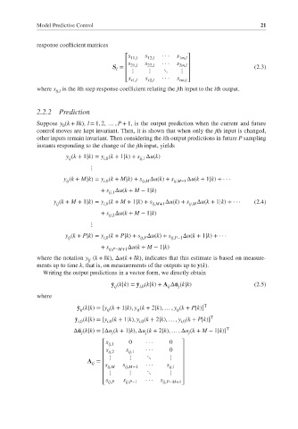
response coefficient matrices
⎡s 11,l s 12,l ··· s 1m,l⎤
⎢s 21,l s 22,l ··· s 2m,l ⎥
S = ⎢ ⋮ ⋮ ⋱ ⋮ ⎥ (2.3)
l
⎢ ⎥
⎣s r1,l s r2,l ··· s rm,l ⎦
where s is the lth step response coefficient relating the jth input to the ith output.
ij,l

2.2.2 Prediction
Suppose y (k + l|k), l = 1, 2, … , P + 1, is the output prediction when the current and future
0
control moves are kept invariant. Then, it is shown that when only the jth input is changed,
other inputs remain invariant. Then considering the ith output predictions in future P sampling
instants responding to the change of the jth input, yields
y (k + 1|k)= y (k + 1|k)+ s Δu(k)
ij
ij,1
i,0
⋮
y (k + M|k)= y (k + M|k)+ s Δu(k)+ s Δu(k + 1|k)+···
ij i,0 ij,M ij,M−1
+ s Δu(k + M − 1|k)
ij,1
y (k + M + 1|k)= y (k + M + 1|k)+ s ij,M+1 Δu(k)+ s ij,M Δu(k + 1|k)+··· (2.4)
ij
i,0
+ s Δu(k + M − 1|k)
ij,2
⋮
y (k + P|k)= y (k + P|k)+ s Δu(k)+ s Δu(k + 1|k)+···
ij i,0 ij,P ij,P−1
+ s ij,P−M+1 Δu(k + M − 1|k)
where the notation y (k + l|k), Δu(k + l|k), indicates that this estimate is based on measure-
ij
ments up to time k, that is, on measurements of the outputs up to y(k).
Writing the output predictions in a vector form, we directly obtain

̃ y (k|k)= ̃ y (k|k)+ A Δ̃ u (k|k) (2.5)
ij
ij
j
i,0
where
̃ y (k|k)=[y (k + 1|k), y (k + 2|k), … , y (k + P|k)] T
ij ij ij ij
̃ y (k|k)=[y (k + 1|k), y (k + 2|k), … , y (k + P|k)] T
i,0 i,0 i,0 i,0
T
Δ̃ u (k|k)=[Δu (k + 1|k), Δu (k + 2|k), … , Δu (k + M − 1|k)]
j j j j
⎡s ij,1 0 ··· 0 ⎤
⎢ s s ··· 0 ⎥
ij,2 ij,1
⎢ ⋮ ⋮ ⋱ ⋮ ⎥
A = ⎢ ⎥
ij
⎢s ij,M s ij,M−1 ··· s ij,1 ⎥
⎢ ⋮ ⋮ ⋱ ⋮ ⎥
⎢ ⎥
⎣ s ij,P s ij,P−1 ··· s ij,P−M+1⎦