Page 49 - Distributed model predictive control for plant-wide systems

Model Predictive Control 23

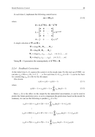
At each time k, implement the following control move:
Δu = DE (k) (2.10)
0
where
D = L(A WA + R) A W
̃ T ̃ ̃
̃ −1 ̃ T ̃
⎡ ··· ⎤
⎢ ··· ⎥
L = ∈ ℝ m×mM
⎢ ⋮ ⋮ ⋱ ⋮ ⎥
⎣ ··· ⎦
⎢
⎥
[ ] M
= 1 0 ··· 0 ∈ ℝ
A simple selection of W and R is
̃
̃
W = diag{W , W , … , W }
̃
1 2 n
R = diag{R , R , … , R }
̃
1 2 m
W = diag{w , w , … , w }, i ∈{1, 2, … , n}
i i1 i2 iP
R = diag{r , r , … , r }, j ∈{1, 2, … , m}
jM
j
j1
j2
̃ T ̃ ̃
̃
Taking R > 0 guarantees the nonsingularity of A WA + R.
̃
2.2.4 Feedback Correction
At the initial time k = 0, suppose the system is in the steady state. For the start-up of DMC, we
can take y (1|0) = y (0), i = 1, 2, … , n. For each time k > 0, y (k + l|k − 1) can be the basis
i,0 i i,0
for constructing y (k + l|k)forthe ith output.
i,0
Also denote
(k)= y (k)− y (k|k − 1) (2.11)
i
i
i
where
m
∑
y (k|k − 1)= y (k|k − 1)+ s Δu (k − 1) (2.12)
i,0
ij,1
j
i
j=1
Since (k) is the effect on the output by the unmodeled uncertainties, it can be used to
i
predict the future prediction error, so as to compensate the predictions based on the model. In
summary, we can use the following to predict y (k + l|k):
i,0
m
∑
y (k + 1|k)= y (k + 2|k − 1)+ s Δu (k − 1)+ f (k)
i,0
ij,2
i,0
i,1
j
j=1
⋮
m
∑
y (k + M|k)= y (k + M + 1|k − 1)+ s Δu (k − 1)+ f (k)
i,0 i,0 ij,M+1 j i,M i
j=1
⋮
m
∑
y (k + P|k)= y (k + P|k − 1)+ s ij,P+1 Δu (k − 1)+ f (k)
i,0
i,P i
i,0
j
j=1