Page 53 - Distributed model predictive control for plant-wide systems

Model Predictive Control 27

• the cost function is quadratic,
• the cost function does not penalize particular values of the input vector u(k), but only the
input increments vector, Δu(k), which coincides with that used in the majority of the pre-
dictive control literature,
• constraints are in the form of linear inequalities.

2.3.1 System Model

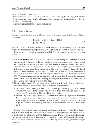
Consider a dynamic time-invariant linear system with measurement disturbances, which is
express as
{
x (k + 1) = Ax(k)+ Bu(k)+ Ed(k)
(2.21)
y(k)= Cx(k)
where x(k)∈ ℝ , y(k)∈ ℝ , u(k)∈ ℝ , and d(k)∈ ℝ n d are state, output, input, and mea-
n y
n x
n u
surable disturbances vector, respectively. A, B, C, D, and E are system coefficient matrices.
There are several methods to obtain the model of (2.21), and two of them are introduced as
follows.
1. Black-box model: Most commonly, it is obtained by performing tests on the plant, which
involve injecting known signals, such as steps, multi-sines, pseudorandom, or others, at
the plant inputs, and recording the resulting plant outputs and the measurable disturbances.
Then the linear time-invariant models can be obtained by using the system identification
techniques, which range from simple curve fitting to sophisticated statistically based
methods. Models obtained in this way are “black-box” models, which represent only the
input–output behavior of the plant, and carry no information about its internal structure
[75–77]. Although the subspace identification method could directly obtain the state space
model, the state of the identified model by the subspace method usually cannot reflect a
real physical state variable in an industrial plant.
2. First-principle model: When a first-principle nonlinear model of the plant is available, the
linear time-invariant model can be obtained by the following methods:
• One way we can do is to approximate these first-principle models by Taylor series. How-
ever, in some cases, if the first-principle model contains nonsmooth elements such as
switches and look-up tables, this method is not appropriate.
• Another very effective procedure is to use the nonlinear model to generate simulation
data by injecting particular signals, such as steps, multi-sines, pseudorandom, or others,
to the first-principle nonlinear model, and then to apply system identification techniques
to get the black-box model using these data, as if they have been obtained from the plant
itself.

The first-principle model refers to a model in which the equations are obtained from knowl-
edge of the underlying physical, chemical, and thermodynamic processes. For motion control,
in most cases, the equations describe that the nonlinear dynamics of an aircraft are accu-
rate, and not very complicated. For complex industrial processes, such first-principle dynamic
models are much more complex and expensive to develop, but this is being done increasingly
commonly.