Page 56 - Distributed model predictive control for plant-wide systems

30 Distributed Model Predictive Control for Plant-Wide Systems

Then, the concatenated predictive model can be expressed as
{
X (k|k) = Hx(k|k)+ GΔU(k|k)+ Fu(k − 1|k − 1)+ VW(k|k)
(2.24)
Y(k|k)= TX(k|k)
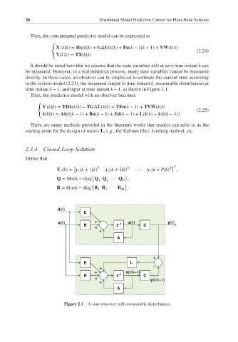
It should be noted here that we assume that the state variables x(k) at very time instant k can
be measured. However, in a real industrial process, many state variables cannot be measured
directly. In these cases, an observer can be employed to estimate the current state according
to the system model (2.21), the measured output in time instant k, measurable disturbances at
time instant k − 1, and input at time instant k − 1, as shown in Figure 2.1.
Then, the predictive model with an observer becomes
{
Y (k|k) = TĤ x(k|k)+ TGΔU(k|k)+ TFu(k − 1)+ TVW(k|k)
(2.25)
̂ x(k|k)= Â x(k|k − 1)+ Bu(k − 1)+ Ed(k − 1)+ L(̂ y(k)− ̂ y(k|k − 1))
There are many methods provided in the literature works that readers can refer to as the
starting point for the design of matrix L, e.g., the Kalman filter, Lunberg method, etc.

2.3.4 Closed-Loop Solution

Define that
[ T ] T
Y (k)= y (k + 1|k) y (k + 2|k) T ··· y (k + P|k) T ,
r r r r
{ }
Q = block − diag Q Q ··· Q P ,
2
1
{ }
R = block − diag R R ··· R M .
1
2
d(k)
E
u(k) + −1 x(k) y(k)
B z C
+
+
A

+
E L
+ −
+ x(k|k−1)
B z −1 C
+
+ y(k|k−1)
A

Figure 2.1 A state observer with measurable disturbances