Page 54 - Distributed model predictive control for plant-wide systems

28 Distributed Model Predictive Control for Plant-Wide Systems

2.3.2 Performance Index

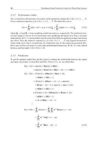
The cost function J(k) penalizes deviations of the prediction outputs ˆ y(k + i|k), i = 1, 2, … , P,
from a reference trajectory y (k + i|k), i = 1, 2, … , P. We define the cost as
r
P M
∑ 2 ∑ 2
J(k)= ||̂ y(k + i|k)− y (k + i|k)|| Q i + ||Δu(k + i − 1|k)|| R i (2.22)
r
i=1 i=1
where Q ≻ 0 and R ≻ 0 are weighting coefficient matrices, respectively. The prediction hori-
i
i
zon has length P, but we do not necessarily start penalizing deviations of y from a set-point
immediately (if P > 1), because there may be some delay between applying an input and seeing
any effect. Thus, the reference trajectory y (k + i|k), i = 1, 2, … , P, may depend on measure-
r
ments made up to time k; in particular, its initial point may be the output measurement y(k).
But it may also be a set-point, or some other predetermined trajectory. M, M < P, is the control
horizon, and that Δu(k + i|k) = 0for i > M.

2.3.3 Prediction

To get the optimal control law, the first step is to deduce the relationship between the output
and input concatenate version Y(k) and U(k). From (2.21), we can obtain that

̂ x(k + 1|k)= Ax(k|k)+ Bu(k|k)+ Ed(k)
= Ax(k|k)+ BΔu(k|k)+ Bu(k − 1|k − 1)+ Ed(k)
2
̂ x(k + 2|k)= A x(k|k)+ ABu(k|k)+ Bu(k + 1|k)
+ AEd(k)+ Ed(k + 1)
̂
2
= A x(k|k)+ AB(u(k − 1|k − 1)+Δu(k|k))
+ B((u(k − 1|k − 1)+Δu(k|k)+Δu(k + 1|k))

+ AEd(k)+ Ed(k + 1)
̂
2
= A x(k|k)+(A + I)BΔu(k|k)+ BΔu(k + 1|k)
+ AEd(k)+ Ed(k + 1)
̂
+(A + I)Bu(k − 1|k − 1)
⋮

P P i
∑ ∑ ∑
l
̂ x(k + P|k)= A x(k|k)+ A j−1 BΔu(k + i − 1|k)
l=1 i=1 j=1
P
∑
Ed(k + h − 1|k)
+ A h−1 ̂
h=1
P
∑ i−1
+ A Bu(k − 1|k − 1) (2.23)
i=1