Page 156 - Dynamic Vision for Perception and Control of Motion

140 5 Extraction of Visual Features

C (m m ) /(2 d ),
˜
0 d d
C 1.5 (m d m d ) / d 2 ,
˜
1
(5.7)
ȥ 0.25 ( m m ),
˜
0 d d
˜
y 0.25 (m m ) d .
˜
0 d d
The linear curva-
ture model can be
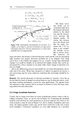
Linear curvature model: y = 0.25 (m +d – m íd )·d
0
C = C + C · s; í d < s < + d P +d m +d computed easily from
1
0
the tangent directions
0
Ȍ íd = arctan(m íd ) § m íd relative to the chord
x d
0
Ȍ -d line and the distance
(2·d) between the
P -d y C = (m +d – m íd )/(2·d)
s 0
íd tangent points. Of
C = 1.5·(m -d + m +d )/d 2
1
course, this distance
m -d
Ȍ = í 0.25·(m íd + m )
has to be chosen such
0 +d
that the angle con-
Figure 5.14. Approximate determination of curvature of a
straint (|ȥ| < 0.2 ra-
slightly curved edge by sub-pixel localization of edge points
and tangent directions: Hermite-interpolation of a third order dian) is not violated.
parabola from two tangent points On smooth curves,
this is always possi-
ble; however, for
large curvatures, the distance d allowed becomes small and the scale for measuring
edge locations and tangent directions probably has to be adapted. Very sharp
curves have to be isolated and jumped over as “corners” having large directional
changes over small arc lengths. In an idealized but simple scheme, they can be ap-
proximated by a Dirac impulse in curvature with a finite change in direction over
zero arc length.
Due to the differencing process unavoidable for curvature determination, the re-
sults tend to be noisy. When basic properties of objects recognized are known, a
post–processing step for noise reduction exploiting this knowledge should be in-
cluded.
Remark: The special advantage of subscale resolution for dynamic vision lies in
the fact that the onset of changes in motion behavior may be detected earlier, yield-
ing better tracking performance, crucial for some applications. The aperture prob-
lem inherent in edge tracking will be revisited in Section 9.5 after the basic track-
ing problem has been discussed.
5.2.3 Edge Candidate Selection
Usually, due to image noise there are many insignificant extreme values in the re-
sulting correlation vector, as can be seen in Figure 5.6. Positioning the threshold
properly (and selecting the mask parameters in general) depends very much on the
scene at hand, as may be seen in Figure 5.15, due to shadow boundaries and scene
noise, the largest gradient values may not be those looked for in the task context
(road boundary). Colinearity conditions (or even edge elements on a smoothly