Page 151 - Dynamic Vision for Perception and Control of Motion

5.2 Efficient Extraction of Oriented Edge Features 135

ference is largest in amplitude, (a) Masks characterized by: (n d n 0 n d )
the gradient over two consecu-
tive mask elements is maxi-
m d = 2; m d = 3; m d = 5; m d = 8
mal.
m d = 17 (Total mask depth)
b) (b) 7 3 7
However, due to local per-
turbations, this need not corre-
(c)
spond to an actual extreme
gradient on the scale of inter-
est. Experience with images
from natural environments has
shown that two additional pa-
rameters may considerably
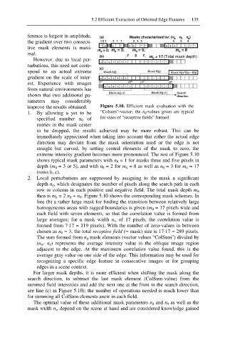
improve the results obtained: Figure 5.10. Efficient mask evaluation with the
1. By allowing a yet to be “Colsum”-vector; the n d -values given are typical
specified number n 0 of for sizes of “receptive fields” formed
entries in the mask center
to be dropped, the results achieved may be more robust. This can be
immediately appreciated when taking into account that either the actual edge
direction may deviate from the mask orientation used or the edge is not
straight but curved; by setting central elements of the mask to zero, the
extreme intensity gradient becomes more pronounced. The rest of Figure 5.10
shows typical mask parameters with n 0 = 1 for masks three and five pixels in
depth (m d = 3 or 5), and with n 0 = 2 for m d = 8 as well as n 0 = 3 for m d = 17
(rows b, c).
2. Local perturbations are suppressed by assigning to the mask a significant
depth n d, which designates the number of pixels along the search path in each
row or column in each positive and negative field. The total mask depth m d
then is m d = 2 n d + n 0. Figure 5.10 shows the corresponding mask schemes. In
line (b) a rather large mask for finding the transition between relatively large
homogeneous areas with ragged boundaries is given (m d = 17 pixels wide and
each field with seven elements, so that the correlation value is formed from
large averages; for a mask width n w of 17 pixels, the correlation value is
formed from 7·17 = 119 pixels). With the number of zero-values in between
chosen as n 0 = 3, the total receptive field (= mask) size is 17·17 = 289 pixels.
The sum formed from n d mask elements (vector values “ColSum”) divided by
(n w· n d) represents the average intensity value in the oblique image region
adjacent to the edge. At the maximum correlation value found, this is the
average gray value on one side of the edge. This information may be used for
recognizing a specific edge feature in consecutive images or for grouping
edges in a scene context.
For larger mask depths, it is more efficient when shifting the mask along the
search direction, to subtract the last mask element (ColSum-value) from the
summed field intensities and add the next one at the front in the search direction,
see line (c) in Figure 5.10); the number of operations needed is much lower than
for summing all ColSum elements anew in each field.
The optimal value of these additional mask parameters n d and n 0 as well as the
mask width n w depend on the scene at hand and are considered knowledge gained