Page 155 - Dynamic Vision for Perception and Control of Motion
P. 155
5.2 Efficient Extraction of Oriented Edge Features 139
the result of a parabolic interpolation for the three points.
Once it is known that the edge is curved – because the edge point at the center
does not lie on the straight line connecting the neighboring edge points – the ques-
tion arises whether the amount of curvature can also be determined with little effort
(at least approximately). This is the case.
5.2.2.3 Approximate Determination of Edge Curvature
When applying a series of equidistant search stripes to an image region, the method
of the previous section yields to each point on the edge also the corresponding edge
direction that is its tangent. Two points and two slopes determine the coefficients
of a third-order polynomial, dubbed Hermite-interpolation after a French mathema-
tician. As a third-order curve, it can have at most one inflection point. Taking the
connecting line (dash-dotted in Figure 5.14) between the two tangent points P -d and
P +d as reference (chord line or secant), a simple linear relationship for a smooth
curve with small angles ȥ relative to the chord line can be derived. Tangent direc-
tions are used in differential-geometry terms, yielding a linear curvature model; the
reference is the slope of the straight line connecting the tangent points (secant). Let
m íd and m +d be the slopes of the tangents at points P íd and P +d respectively; s be the
running variable in the direction of the arc (edge line); and ȥ the angle between the
local tangent and the chord direction (|ȥ| < 0.2 radian so that cos(ȥ) §1).
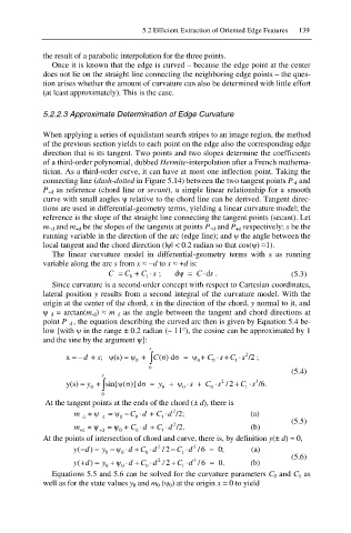
The linear curvature model in differential-geometry terms with s as running
variable along the arc s from x §íd to x § +d is:
C C 0 + C s ; dȥ C ds . (5.3)
1
Since curvature is a second-order concept with respect to Cartesian coordinates,
lateral position y results from a second integral of the curvature model. With the
origin at the center of the chord, x in the direction of the chord, y normal to it, and
ȥ íd = arctan(m -d) § m íd as the angle between the tangent and chord directions at
point P íd , the equation describing the curved arc then is given by Equation 5.4 be-
low [with ȥ in the range ± 0.2 radian (~ 11°), the cosine can be approximated by 1
and the sine by the argument ȥ]:
s
0 ³
x = d + ; ȥ(s) s ȥ + C (ı) d ı ȥ 0 + C s+C s 2 /2 ;
0
1
0
(5.4)
s
y(s) = + sin[ȥ(ı)] dı y 0 ȥ s C s 2 /2 Cs /6. 1 3
0 ³
y
0
0
0
At the tangent points at the ends of the chord (± d), there is
m | d ȥ = ȥ d 0 C d + C d 2 /2; (a)
0
1
(5.5)
m | +d ȥ = ȥ + C d + C d 2 /2. (b)
1
0
0
+d
At the points of intersection of chord and curve, there is, by definition y(± d) = 0,
( y ) d y 0 ȥ d C d 2 / 2 C d 3 /6 0; (a)
0
0
1
(5.6)
( y ) d y ȥ d C d 2 / 2 C d 3 /6 0. (b)
0 0 0 1
Equations 5.5 and 5.6 can be solved for the curvature parameters C 0 and C 1 as
well as for the state values y 0 and m 0 (ȥ 0) at the origin x = 0 to yield

