Page 147 - Dynamic Vision for Perception and Control of Motion

5.2 Efficient Extraction of Oriented Edge Features 131

size expected (domain knowledge) or known from previous images, thereby reduc-
ing the computational load.
It can be seen from Figure 5.4 that the same width at scaled distance 5 (depth in
viewing direction, 31 pixels wide) is reduced to about 2 pixels at a scaled distance
of 20. Clearly, features in the real world will change in appearance accordingly! In
the stripe-based method to be discussed in Section 5.3, these facts may be taken
into account by proper parameter specifica-
tion depending on the actual situation en- Crossroad, area-based
Measurement model
countered. At longer distances, often the Distant
center of homogeneous regions in a stripe road
can be more reliably detected than the exact Area-based
position of edges belonging to the same re-
detection
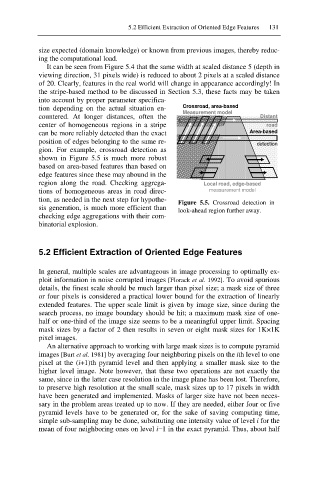
gion. For example, crossroad detection as
shown in Figure 5.5 is much more robust
based on area-based features than based on
edge features since these may abound in the
region along the road. Checking aggrega- Local road, edge-based
tions of homogeneous areas in road direc- measurement model
tion, as needed in the next step for hypothe- Figure 5.5. Crossroad detection in
sis generation, is much more efficient than
look-ahead region further away.
checking edge aggregations with their com-
binatorial explosion.

5.2 Efficient Extraction of Oriented Edge Features

In general, multiple scales are advantageous in image processing to optimally ex-
ploit information in noise corrupted images [Florack et al. 1992]. To avoid spurious
details, the finest scale should be much larger than pixel size; a mask size of three
or four pixels is considered a practical lower bound for the extraction of linearly
extended features. The upper scale limit is given by image size, since during the
search process, no image boundary should be hit; a maximum mask size of one-
half or one-third of the image size seems to be a meaningful upper limit. Spacing
mask sizes by a factor of 2 then results in seven or eight mask sizes for 1K×1K
pixel images.
An alternative approach to working with large mask sizes is to compute pyramid
images [Burt et al. 1981] by averaging four neighboring pixels on the ith level to one
pixel at the (i+1)th pyramid level and then applying a smaller mask size to the
higher level image. Note however, that these two operations are not exactly the
same, since in the latter case resolution in the image plane has been lost. Therefore,
to preserve high resolution at the small scale, mask sizes up to 17 pixels in width
have been generated and implemented. Masks of larger size have not been neces-
sary in the problem areas treated up to now. If they are needed, either four or five
pyramid levels have to be generated or, for the sake of saving computing time,
simple sub-sampling may be done, substituting one intensity value of level i for the
mean of four neighboring ones on level ií1 in the exact pyramid. Thus, about half