Page 39 - Dynamic Vision for Perception and Control of Motion

2.1 Three-dimensional (3-D) Space and Time 23

Space flight and lighting from our sun and moon extend up to 150 million km as
a characteristic range (radius of Earth orbit).
Visible stars are far beyond these distances (not of interest here).
Is it possible to find one single type of representation covering the entire range?
This is certainly not achievable by methods using grids of different scales as often
done in “artificial intelligence”- approaches. Rather, the approach developed in
computer graphics with normalized shape descriptions and overall scaling factors
is the prime candidate. Homogeneous coordinates as introduced by [Roberts 1965,
Blinn 1977] also allow, besides scaling, incorporating the perspective mapping
process in the same framework. This yields a unified approach for computer vision
and computer graphics; however, in computer vision, many of the variables enter-
ing the homogeneous transformation matrices are the unknowns of the problem. A
direct application of the methods from computer graphics is thus impossible, since
the inversion of perspective projection is a strongly nonlinear problem with the
need to recover one space component completely lost in mapping (range).
Introducing strong constraints to the temporal evolution of (3-D) spatial trajec-
tories, however, allows recovering part of the information lost by exploiting first-
order derivatives. This is the big advantage of spatiotemporal models and recursive
least-squares estimation over direct perspective inversion (computational vision).
The Jacobian matrix of this approach to be discussed throughout the text plays a vi-
tal role in the 4-D approach to image sequence understanding.
Before this can be fully appreciated, the chain of coordinate transformations
from an object-centered feature distribution for each object in 3-D space to the
storage of the 2-D image in computer memory has to be understood.

2.1 Three-dimensional (3-D) Space and Time

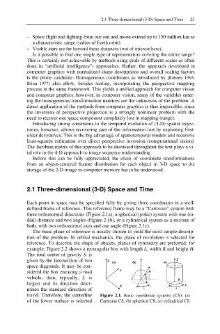
Each point in space may be specified fully by giving three coordinates in a well-
defined frame of reference. This reference frame may be a “Cartesian” system with
three orthonormal directions (Figure 2.1a), a spherical (polar) system with one (ra-
dial) distance and two angles (Figure 2.1b), or a cylindrical system as a mixture of
both, with two orthonormal axes and one angle (Figure 2.1c).
The basic plane of reference is usually chosen to yield the most simple descrip-
tion of the problem: In orbital mechanics, the plane of revolution is selected for
reference. To describe the shape of objects, planes of symmetry are preferred; for
example, Figure 2.2 shows a rectangular box with length L, width B and height H.
The total center of gravity S t is
given by the intersection of two Z Z
(a) (b) (c)
space diagonals. It may be con-
sidered the box encasing a road Y R
vehicle; then, typically, L is /
R
largest and its direction deter-
X D
mines the standard direction of O
travel. Therefore, the centerline Figure 2.1. Basic coordinate systems (CS): (a)
of the lower surface is selected Cartesian CS, (b) spherical CS, (c) cylindrical CS