Page 83 - Dynamic Vision for Perception and Control of Motion

3.3 Perceptual Capabilities 67

measured. Experiments with inexpensive rate sensors have shown that perturba-
tions in the pitch angle amplitude of optical rays can be reduced by at least one or-
der of magnitude this way (inertial angular rate feedback, see Figure 12.2).
Driving cross-country on rough terrain may lead to pitch amplitudes of ± 20° at
frequencies up to more than 1 Hz. Pitch rates up to ~ 100°/s may result. In addition
to pitch, bank and yaw angles may also have large perturbations. Visual orientation
with cameras mounted directly on the vehicle body will be difficult (if not
impossible) under these conditions. This is especially true since vision, usually, has
a rather large delay time (in the tenths of a second range) until the situation has
been understood purely based on visual perception.
If a subject’s body motion can be perceived by a full set of inertial sensors
(three linear accelerometers and three rate sensors), integration of these sensor sig-
nals as in “strap-down navigation” will yield good approximations of the true an-
gular position with little time delay (see Figure 12.1). Note however, that for cam-
eras mounted directly on the body, the images always contain the effects of motion
blur due to integration time of the vision sensors! On the other hand, the drift errors
accumulating from inertial integration have to be handled by visual feedback of
low-pass filtered signals from known stationary objects far away (like the horizon).
In a representation with a scene tree as discussed in Chapter 2, the reduction in
complexity by mounting the cameras directly on the car body is only minor. Once
the computing power has been there for handling this concept, there is almost no
advantage in data processing compared to active vision with gaze control. Hard-
ware costs and space for mounting the gaze control system are the issues keeping
most developers away from taking advantage of a vertebrate type eye. As soon as
high speeds with large look-ahead distances or dynamic maneuvering are required,
the visual perception capabilities of cameras mounted directly on body will no
longer be sufficient.
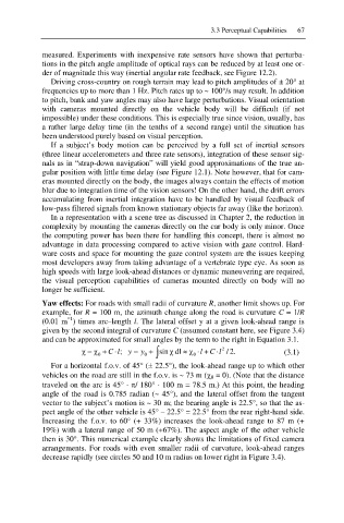
Yaw effects: For roads with small radii of curvature R, another limit shows up. For
example, for R = 100 m, the azimuth change along the road is curvature C = 1/R
í1
(0.01 m ) times arc–length l. The lateral offset y at a given look-ahead range is
given by the second integral of curvature C (assumed constant here, see Figure 3.4)
and can be approximated for small angles by the term to the right in Equation 3.1.
Ȥ Ȥ 0 Cl ; y y 0 ³ sin Ȥ dl | Ȥ l C l 2 /2. (3.1)
˜
˜
˜

0
For a horizontal f.o.v. of 45° (r 22.5°), the look-ahead range up to which other
vehicles on the road are still in the f.o.v. is ~ 73 m (F 0 = 0). (Note that the distance
traveled on the arc is 45° · S/ 180° · 100 m = 78.5 m.) At this point, the heading
angle of the road is 0.785 radian (~ 45°), and the lateral offset from the tangent
vector to the subject’s motion is ~ 30 m; the bearing angle is 22.5°, so that the as-
pect angle of the other vehicle is 45° – 22.5° = 22.5° from the rear right-hand side.
Increasing the f.o.v. to 60° (+ 33%) increases the look-ahead range to 87 m (+
19%) with a lateral range of 50 m (+67%). The aspect angle of the other vehicle
then is 30°. This numerical example clearly shows the limitations of fixed camera
arrangements. For roads with even smaller radii of curvature, look-ahead ranges
decrease rapidly (see circles 50 and 10 m radius on lower right in Figure 3.4).