Page 90 - Dynamic Vision for Perception and Control of Motion

3 Subjects and Subject Classes
74

one obtains
dX/dt = dX /dt + dx/dt . (3.4)
N
The resulting sets of differential equations for the nominal trajectory then are
dX /dt = f ( X , U , p , t ) , (3.5)
N
N
N
and for the linearized perturbation system,
dx/dt = F x + G u + v'(t), (3.6)
˜
˜
with F = df / dX| ; G = df / dU| N
N
as (n × n)- respectively (n × r)-matrices and v’(t) an additive noise-term. In systems
with feedback components, the local feedback component simultaneously ensures
(or at least improves) the validity of the linearized model, if the loop is stable.
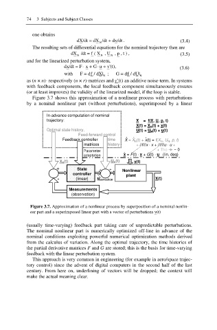
Figure 3.7 shows this approximation of a nonlinear process with perturbations
by a nominal nonlinear part (without perturbations), superimposed by a linear
In-advance computation of nominal
trajectory: X = f(X, U, p, t)
X(t) = X N (t) + x(t)
Optimal state history, U(t) = U N (t) + u(t)
Feed-forward control . . .
Feedback controller time X = X N (t) + x(t) = f(X N , U N , p, t)
matrices history + wf/wx ˜ x + wf/wu ˜ u +
Parameter . + Tho ~ 0
adaptation x = F(t) ˜ x + G(t) ˜ u (lin. deq)
X N (t) U N (t) v(t)
+ State + + Nonlinear
controller plant
- (linear) u correction X(t)
Measurements
(observation)

Figure 3.7. Approximation of a nonlinear process by superposition of a nominal nonlin-
ear part and a superimposed linear part with a vector of perturbations v(t)

(usually time-varying) feedback part taking care of unpredictable perturbations.
The nominal nonlinear part is numerically optimized off-line in advance of the
nominal conditions exploiting powerful numerical optimization methods derived
from the calculus of variation. Along the optimal trajectory, the time histories of
the partial derivative matrices F and G are stored; this is the basis for time-varying
feedback with the linear perturbation system.
This approach is very common in engineering (for example in aero/space trajec-
tory control) since the advent of digital computers in the second half of the last
century. From here on, underlining of vectors will be dropped; the context will
make the actual meaning clear.