Page 93 - Dynamic Vision for Perception and Control of Motion

3.4 Behavioral Capabilities for Locomotion 77

of the environment due to pitching effects must correspond to accelerations sensed.
A downward pitch angle leads to a shift of all features upward in the images. [In
humans, perturbations destroying this correspondence may lead to “motion sick-
ness”. This may also originate from different delay times in the sensor signal paths
(e.g., “simulator sickness”) or from additional rotational motion around other axes
disturbing the vestibular apparatus in humans which delivers the inertial data.]
For a human driver, the direct feedback of inertial data after applying one of the
longitudinal controls is essential information on the situation encountered. For ex-
ample, when the deceleration felt after brake application is much lower than ex-
pected the friction coefficient to the ground may be smaller than expected (slippery
or icy surface). With a highly powered car, failing to meet the expected accelera-
tion after a positive change in throttle setting may be due to wheel spinning. If a ro-
tation around the vertical axis occurs during braking, the wheels on the left- and
right-hand sides may have encountered different frictional properties of the local
ground. To counteract this immediately, the system should activate lateral control
with steering, generating the corresponding countertorque.

3.4.2.2 Lateral Control of Ground Vehicles

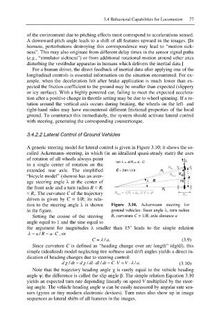
A generic steering model for lateral control is given in Figure 3.10; it shows the so-
called Ackermann–steering, in which (in an idealized quasi-steady state) the axes
of rotation of all wheels always point
tan O = a/R r = a · C O
to a single center of rotation on the
R fin
extended rear axle. The simplified C = (tan O)/a R f
“bicycle model” (shown) has an aver- R fout V cg a
age steering angle Ȝ at the center of O R cg
the front axle and a turn radius R § R f
R r
§ R r. The curvature C of the trajectory R fout = ¥(R r + b Tr /2 )² + a² b Tr
driven is given by C = 1/R; its rela-
tion to the steering angle Ȝ is shown Figure 3.10. Ackermann steering for
in the figure. ground vehicles: Steer angle O, turn radius
Setting the cosine of the steering R, curvature C = 1/R, axle distance a
angle equal to 1 and the sine equal to
the argument for magnitudes Ȝ smaller than 15° leads to the simple relation
O / aR a C , or
˜
a
C O /. (3.9)
Since curvature C is defined as “heading change over arc length” (dȤ/dl), this
simple (idealized) model neglecting tire softness and drift angles yields a direct in-
dication of heading changes due to steering control:
˜
d / dt F dF / dl dl dt ˜ / C V V ˜ O a /. (3.10)
Note that the trajectory heading angle Ȥ is rarely equal to the vehicle heading
angle ȥ; the difference is called the slip angle ȕ. The simple relation Equation 3.10
yields an expected turn rate depending linearly on speed V multiplied by the steer-
ing angle. The vehicle heading angle ȥ can be easily measured by angular rate sen-
sors (gyros or tiny modern electronic devices). Turn rates also show up in image
sequences as lateral shifts of all features in the images.