Page 96 - Dynamic Vision for Perception and Control of Motion

3 Subjects and Subject Classes
80

These numbers may serve as a first reference for grasping the real-world effects
when the corresponding control output is used with a real vehicle in testing. In Sec-
tion 3.4.5, some of the most essential effects stemming from systems dynamics ne-
glected here will be discussed.

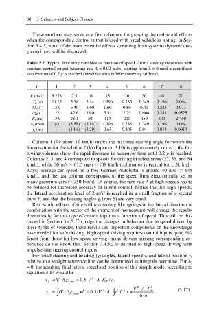
Table 3.2. Typical final state variables as function of speed V for a steering maneuver with
constant control output (steering-rate A = 0.02 rad/s) starting from Ȝ = 0 until a centrifugal
acceleration of 0.2 g is reached (idealized with infinite cornering stiffness)

0 1 2 3 4 5 6 7 8
V (m/s) 5.278 7.5 10 15 20 30 40 70
T 2 (s) 11.27 5.58 3.14 1.396 0.785 0.349 0.196 0.064
ǻȜ f (˚) 12.9 6.40 3.60 1.60 0.89 0.40 0.225 0.073
ǻȤ f (˚) 122. 42.6 18.0 5.33 2.25 0.666 0.281 0.0525
R f (m) 13.9 28.1 50 113 200 450 800 2.450
v f (m/s) (-) (5.58) (3.14) 1.396 0.785 0.349 0.196 0.064
y f (m) - (10.4) (3.29) 0.65 0.205 0.041 0.013 0.0014

Column 1 (for about 19 km/h) marks the maximal steering angle for which the
linearization for the relation C(Ȝ) (Equation 3.10) is approximately correct; the fol-
lowing columns show the rapid decrease in maneuver time until 0.2 g is reached.
Columns 2, 3, and 4 correspond to speeds for driving in urban areas (27, 36, and 54
km/h), while 30 m/s § 67.5 mph § 108 km/h (column 6) is typical for U.S. high-
ways; average car speed on a free German Autobahn is around 40 m/s (§ 145
km/h), and the last column corresponds to the speed limit electronically set in
many premium cars (§ 250 km/h). Of course, the turn rate A at high speeds has to
be reduced for increased accuracy in lateral control. Notice that for high speeds,
the lateral acceleration level of 2 m/s² is reached in a small fraction of a second
(row 3) and that the heading angles Ȥ f (row 5) are very small.
Real-world effects of tire stiffness (acting like springs in the lateral direction in
combination with the vector of the moment of momentum) will change the results
dramatically for this type of control input as a function of speed. This will be dis-
cussed in Section 3.4.5. To judge the changes in behavior due to speed driven by
these types of vehicles, these results are important components of the knowledge
base needed for safe driving. High-speed driving requires control inputs quite dif-
ferent from those for low-speed driving; many drivers missing corresponding ex-
perience do not know this. Section 3.4.5.2 is devoted to high-speed driving with
impulse-like steering control inputs.
For small steering and heading (Ȥ) angles, lateral speed v f and lateral position y f
relative to a straight reference line can be determined as integrals over time. For Ȝ 0
= 0, the resulting final lateral speed and position of this simple model according to
Equation 3.14 would be
2
v V ˜'F 0.5 V ˜ A T 2 / .
˜
a
˜
f ramp SR
2
V ˜˜ 3 (3.17)
A T
2
y f ³ (V ˜ ' F ramp )dt 0.5 V ˜ ˜ 2 A ˜ ³ t dt / a = 6 a SR .
˜