Page 97 - Dynamic Vision for Perception and Control of Motion

3.4 Behavioral Capabilities for Locomotion 81

Row 7 (second from the bottom) in Table 3.2 shows lateral speed v f and row 8
lateral distance y f traveled during the maneuver. Note that for speeds V < 10 m/s
(columns 1 to 3), the heading angle (row 5) is so large that computation with the
linear model (Equation 3.17) is no longer valid (see terms in brackets in the dotted
area at bottom left of the table). On the other hand, for higher speeds (> § 30 m/s),
both lateral speed and position remain quite small when the acceleration limit is
reached; at top speed (last column), they remain close to zero. This indicates again
quite different behavior of road vehicles in the lower and upper speed ranges. The
full nonlinear relation replacing Equation 3.17 for large heading angles is, with
Equation 3.13b,
˜
() V ˜
˜
˜
vt sin(ǻȤ ) V ˜ sin(0.5 V A t 2 / ) . (3.18)
a
ramp
Since the cosine of the heading angle can no longer be approximated by 1, there
is a second equation for speed and distances in the original x-direction:

'
˜
˜
a

˜
dx / dt V ˜ cos( F ramp ) V ˜ cos(0.5 V A t 2 / ) . (3.19)
The time integrals of these equations yield the lateral and longitudinal positions
for larger heading angles as needed in curve steering; this will not be followed
here. Instead, to understand the consequences of one of the simplest maneuvers in
lateral control, let us adjoin a negative
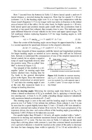
Steer angle O (state)
ramp of equal magnitude directly after A O max = A ·T SR
the positive ramp. This so-called “dou- 1 2
blet” is shown in Figure 3.12. 0 0 Time/T SR
The integral of this doublet is a tri- T SR T SI = 2 ·T SR
-A Steer rate dO/dt
angular “pulse” in steering angle time
(= piecewise constant control input (doublet))
history (dashed line). Scaling time by
T SR leads to the general description Figure 3.12. Doublet in constant steering
given in the figure. Since the maneuver rate U ff (t) = dO/dt as control time history
is locally symmetrical at around point over two periods T SR with opposite sign ±
“1” and since the steering angle is zero A yields a “pulse” in steer angle for head-
at the end, this maneuver leads to a ing change
change in heading direction.
Pulses in steering angle: Mirroring the steering angle time history at T SR = T 2
(when a lateral acceleration of 0.2 g is reached), that is, applying a constant nega-
tive steering rate –A from T 2 to 2T 2 yields a heading change maneuver (idealized)
with maximum lateral acceleration of § 2 m/s².
The steering angle is zero at the end, and the heading angle is twice the value
given in row 5 of Table 3.2 for infinite tire stiffness. From column 2, row 5 it can
be seen that for a speed slightly lower than 7.5 m/s § 25 km/h a 90°-turn should re-
sult with a minimal turn radius of about 28 m (row 6). For exact computation of the
trajectory driven, the sine– and cosine–effects of the heading angle Ȥ (according to
Equations 3.18/3.19) have to be taken into account.
For speeds higher than 50 km/h (§ 14 m/s), all angles reached with a “pulse”–
maneuver in steering and moderate maximum lateral acceleration will be so small
that Equation 3.17 is valid. The last two rows in Table 3.2 indicate for this speed
range that a driving phase with constant Ȝ f (and thus constant lateral acceleration)
over a period of duration IJ should be inserted at the center of the pulse to decrease
the time for lane changing (lane width is typically 2.5 to 3.8 m) achievable by a