Page 281 - Dynamics and Control of Nuclear Reactors

APPENDIX E Frequency response analysis of linear systems 283

Im G(jw)

|G(jw)|

φ(ω)
0 Re G(jw)
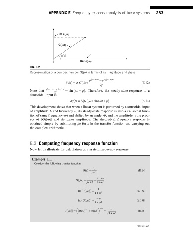
FIG. E.2
Representation of a complex number G(jω) in terms of its magnitude and phase.

e j ωt + φÞ e j ωt + φÞ
ð
ð
j
ð
δytðÞ ¼ Α GjωÞj (E.12)
2j
ð
ð
Note that e j ωt + φÞ e j ωt + φÞ ¼ sin ωt + φÞ. Therefore, the steady-state response to a
ð
2j
sinusoidal input is
δytðÞ ¼ Α GjωÞjsin ωt + φÞ (E.13)
ð
j
ð
This development shows that when a linear system is perturbed by a sinusoidal input
of amplitude A and frequency ω, its steady-state response is also a sinusoidal func-
tion of same frequency (ω) and shifted by an angle, Φ, and the amplitude is the prod-
uct of jG(jω)j and the input amplitude. The theoretical frequency response is
obtained simply by substituting jω for s in the transfer function and carrying out
the complex arithmetic.
E.2 Computing frequency response function
Now let us illustrate the calculation of a system frequency response.

Example E.1
Consider the following transfer function:
1
GsðÞ ¼ (E.14)
s +1
1 1 jω
GjωÞ ¼ ¼
ð
jω +1 1+ ω 2
1
f
ð
Re GjωÞg ¼ (E.15a)
1+ ω 2
ω
ð
f
Im GjωÞg ¼ (E.15b)
1+ ω 2
1=2
1
2 2
p
j GjωÞj ¼ ð ReGÞ +ImGð Þ ¼ ffiffiffiffiffiffiffiffiffiffiffiffi (E.16)
ð
1+ ω 2
Continued