Page 284 - Dynamics and Control of Nuclear Reactors

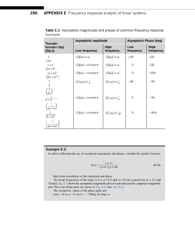
286 APPENDIX E Frequency response analysis of linear systems

Table E.1 Asymptotic magnitudes and phases of common frequency response
functions.
Asymptotic amplitude Asymptotic Phase (deg)
Transfer
function G(s) High Low High
(G(jω)) Low frequency frequency frequency frequency
s jG(jω)j∝ω jG(jω)j∝ω +90 +90
ð jωÞ
s + a jG(jω)j¼constant jG(jω)j∝ω 0 +90
ð jω + aÞ
n jG(jω)j∝ω n
ð s + aÞ jG(jω)j¼constant 0 +90n
n
ð jω + aÞ
1 GjωÞj∝ 1 GjωÞj∝ 1 90 90
ð
ð
j
ω j ω
s
1

jω
1 jG(jω)j¼constant GjωÞj∝ 1 0 90
s + a j ð ω
1

jω + a
1 jG(jω)j¼constant j GjωÞj∝ 1 0 90n
ð
n ω n
ð s + aÞ
1

n
ð jω + aÞ
Example E.2
In order to illustrate the use of asymptotic magnitudes and phases, consider the transfer function.

ð s +1Þ
GsðÞ ¼ (E.24)
ð
ð s +0:1Þ s +10Þ
Each term contributes to the magnitude and phase.
The break frequencies of the terms (s+1), (s+0.1) and (s+10) are respectively at 1, 0.1 and
10rad/s. Fig. E.3 shows the asymptotic magnitude plots of each term and the composite magnitude
plot. The exact Bode plots are shown in Fig. E.4. (See Fig. E.5.)
The asymptotic values of the phase angle are:
φ(ω)!0as ω!0, φ(ω)! 90deg for large ω