Page 279 - Dynamics and Control of Nuclear Reactors

APPENDIX

Frequency response

analysis of linear systems E

E.1 Frequency response theory
The frequency response of a linear time-invariant system is defined as the response of
a selected system output resulting from a sinusoidal perturbation in a selected system
input. The output of a linear system to a sinusoidal input is also a sinusoidal function
with the same frequency as the input sinusoid, but shifted by phase angle, Φ. The
ratio of the amplitude of the output sinusoidal function to the amplitude of the input
sinusoidal function, and the phase angle completely define the frequency response of
the system. After perturbing the system by a sine function of a certain frequency, an
initial, non-sinusoidal output occurs. After initial transient components decay, a con-
tinuing sinusoidal output occurs. This approach is valid only for stable systems; that
is for systems with all the poles of the transfer function with negative real parts.
The frequency response function is widely used in the study of linear systems, in
system design to achieve desired characteristics, and in the stability analysis of linear
systems. Certain frequency domain parameters can be directly related to system char-
acteristics in the time domain. In addition, the frequency domain analysis can provide
quick insight into the dynamic nature of a system by interpreting the significance of the
magnitude and/or phase in certain frequency bands. The basic contributions to this area
ofsystemsanalysisweremadebyBode,Nyquist,Nichols,andothers[1].Bodeplotsare
themostcommongraphicaldepictionsofasystem’sfrequencyresponse.Theyshowthe
response magnitude versus frequency (plotted on a log-log scale); and phase angle ver-
sus frequency (plotted on a semi-log scale) with the phase angle in degrees.
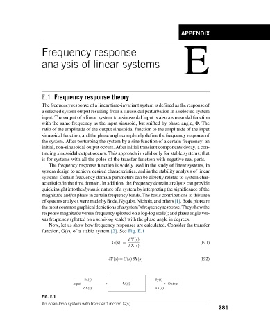
Now, let us show how frequency responses are calculated. Consider the transfer
function, G(s), of a stable system [2]. See Fig. E.1

δYsðÞ
GsðÞ ¼ (E.1)
δXsðÞ
δYsðÞ ¼ GsðÞδXsðÞ (E.2)

dx(t) dy(t)
Input G(s) Output
dX(s) dY(s)

FIG. E.1
An open-loop system with transfer function G(s).
281