Page 274 - Dynamics and Control of Nuclear Reactors

276 APPENDIX D Laplace transforms and transfer functions

The input and output are denoted by δx(t) and δy(t), respectively. The corre-
sponding Laplace transforms are δX(s) and δY(s). The transfer function, G(s), is
defined as the ratio between the Laplace transform of the output and the Laplace
transform of the input.

δYsðÞ
GsðÞ (D.23)
δXsðÞ
In general, the numerator (order m) and denominator (order n) of the transfer func-
tion are polynomials in ‘s’
ð s z 1 Þ s z 2 Þ… s z m Þ
ð
ð
GsðÞ ¼ (D.24)
ð
ð
ð s p 1 Þ s p 2 Þ… s p n Þ
The parameters {p 1 , p 2 , …, p n } are called the poles of G(s). The parameters {z 1 , z 2 ,
…, z m } are called the zeros of G(s). If r of the poles have the same value, then that
th
pole is called an r -order pole. In general, the poles and zeros of G(s) are complex
numbers. It is more common for the poles to be complex values than the zeros,
because the poles of G(s) represent the system dynamics. Also, the order of the
denominator polynomial is always greater than the order of the numerator polyno-
mial. The transfer function reflects the basic characteristics of a system (such as a
differential equation) and is not dependent on initial conditions.

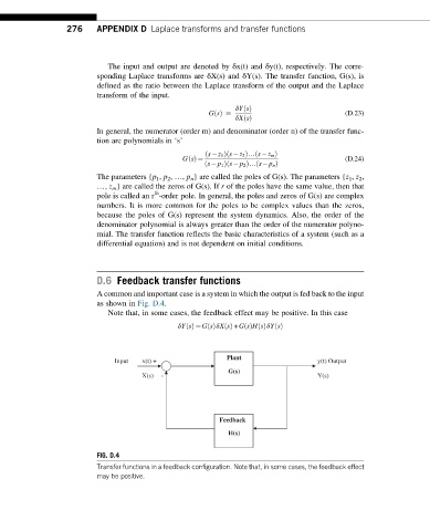
D.6 Feedback transfer functions

A common and important case is a system in which the output is fed back to the input
as shown in Fig. D.4.
Note that, in some cases, the feedback effect may be positive. In this case

δYsðÞ ¼ GsðÞδXsðÞ + GsðÞHsðÞδYsðÞ

Plant
Input x(t) + y(t) Output
G(s)
X(s) - Y(s)

Feedback
H(s)

FIG. D.4
Transfer functions in a feedback configuration. Note that, in some cases, the feedback effect
may be positive.