Page 273 - Dynamics and Control of Nuclear Reactors

APPENDIX D Laplace transforms and transfer functions 275

Solution
Take the Laplace transform of both sides of Eq. (D.18). Use Table D.1 for appropriate transforms
2
s XsðÞ sx 0ðÞ _ x 0ðÞ +3 sX sðÞ x 0ðÞ½ Š +2XsðÞ ¼ FsðÞ
With F(s)¼1/s and zero initial conditions, the above simplifies as
FsðÞ 1
XsðÞ ¼ ¼
2
s +3s +2 ss +1Þ s +2Þ
ð
ð
Express X(s) in the partial fraction form as
1 k 1 k 2 k 3
XsðÞ ¼ ¼ + + (D.19)
ð
ð
ss +1Þ s +2Þ s s +1 s +2
Apply the following steps successively to solve for the constants k 1 ,k 2 , and k 3 .
Multiply both sides of Eq. (D.19) by s, set s¼0, and solve for k 1 . Multiply both sides of
Eq. (D.19) by (s+1), set s¼ 1, and solve for k 2 . Multiply both sides of Eq. (D.19) by (s+2),
set s¼ 2, and solve for k 3 . The numerical values of k 1 ,k 2 , and k 3 are shown in Eq. (D.20)
1 1
k 1 ¼ , k 2 ¼ 1, k 3 ¼ : (D.20)
2 2
Thus X(s) simplifies as
1 1 1
XsðÞ ¼ + (D.21)
2s s +1 2 s +2Þ
ð
To find x(t), take the inverse Laplace transform of the three terms in Eq. (D.21). See Table D.1
for Laplace transform pairs. Thus,
1 1
t
xtðÞ ¼ e + e 2t (D.22)
2 2
Note that Eq. (D.22) satisfies the assumed zero initial conditions
1 1
x 0ðÞ ¼ 1+ ¼ 0
2 2
dx
t
¼ e e 2t and _x 0ðÞ ¼ 0
dt
1
One last point to note—the steady-state value of x(t), as t ! ∞,isx ss tðÞ ¼
2
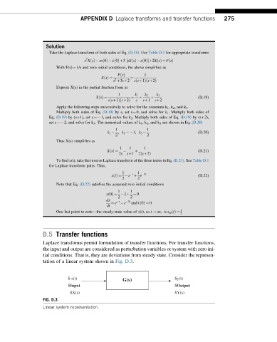
D.5 Transfer functions
Laplace transforms permit formulation of transfer functions. For transfer functions,
the input and output are considered as perturbation variables or system with zero ini-
tial conditions. That is, they are deviations from steady state. Consider the represen-
tation of a linear system shown in Fig. D.3.

x(t) G(s) y(t)
Input Output
X(s) Y(s)
FIG. D.3
Linear system representation.