Page 270 - Dynamics and Control of Nuclear Reactors

272 APPENDIX D Laplace transforms and transfer functions

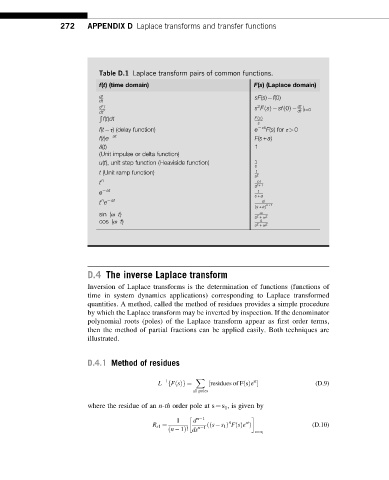
Table D.1 Laplace transform pairs of common functions.
f(t) (time domain) F(s) (Laplace domain)
df sF(s) f(0)
dt
df
2
d f 2 s FsðÞ sf 0ðÞ j
dt 2 dt t¼0
Ð
f(t)dt FsðÞ
s
f(t τ) (delay function) e τs F(s) for τ>0
f(t)e at F(s+a)
δ(t) 1
(Unit impulse or delta function)
u(t), unit step function (Heaviside function) 1
s
t (Unit ramp function) 1
s 2
t n n!
s n +1
e at 1
s + a
n at
t e n!
n +1
ð s + aÞ
ω
sin (ω t) s 2 + ω 2
cos (ω t) s
s 2 + ω 2

D.4 The inverse Laplace transform
Inversion of Laplace transforms is the determination of functions (functions of
time in system dynamics applications) corresponding to Laplace transformed
quantities. A method, called the method of residues provides a simple procedure
by which the Laplace transform may be inverted by inspection. If the denominator
polynomial roots (poles) of the Laplace transform appear as first order terms,
then the method of partial fractions can be applied easily. Both techniques are
illustrated.

D.4.1 Method of residues

X
1 st
L f FsðÞg ¼ ½ residues of F sðÞe Š (D.9)
all poles
where the residue of an n-th order pole at s¼s 1 , is given by
n 1
1 d n st
R s1 ¼ n 1 ð ð s s 1 Þ FsðÞe Þ (D.10)
ð n 1Þ! ds
s¼s 1