Page 272 - Dynamics and Control of Nuclear Reactors

274 APPENDIX D Laplace transforms and transfer functions

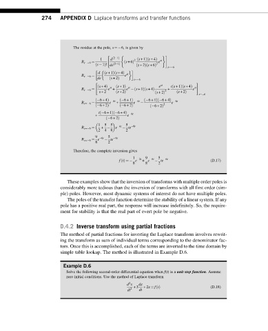
The residue at the pole, s¼ 6, is given by
" ( )#
1 d ð 2 1Þ 2 s +1ð Þ s +4Þ st
ð
R s¼ 6 ¼ ð s +6Þ 2 e
ð s 1Þ! ds ð 2 1Þ ð s +2Þ s +6Þ
ð
s¼ 6

d ð s +1Þ s +4Þ
ð
R s¼ 6 ¼ e st
ds ð s +2Þ
s¼ 6
" #
ð
ð
ð s +4Þ st ð s +1Þ st e st ts +1Þ s +4Þ st
ð
ð
R s¼ 6 ¼ e + e s +1Þ s +4Þ 2 + e
s +2 ð s +2Þ ð s +2Þ ð s +2Þ
s¼ 6
ð 6+4Þ 6t ð 6+ 1Þ 6t ð 6+ 1Þ 6+ 4Þ 6t
ð
R s¼ 6 ¼ e + e 2 e
ð 6+2Þ ð 6+ 2Þ ð 6+ 2Þ
ð
ð
t 6+ 1Þ 6+ 4Þ
+ e 6t
ð 6+ 2Þ

1 5 5 5 6t
R s¼ 6 ¼ + e 6t te
2 4 8 2
9 5
R s¼ 6 ¼ e 6t te 6t
8 2
Therefore, the complete inversion gives
1 9 5
ftðÞ ¼ e 2t + e 6t te 6t (D.17)
8 8 2
These examples show that the inversion of transforms with multiple order poles is
considerably more tedious than the inversion of transforms with all first order (sim-
ple) poles. However, most dynamic systems of interest do not have multiple poles.
The poles of the transfer function determine the stability of a linear system. If any
pole has a positive real part, the response will increase indefinitely. So, the require-
ment for stability is that the real part of evert pole be negative.
D.4.2 Inverse transform using partial fractions
The method of partial fractions for inverting the Laplace transform involves rewrit-
ing the transform as sum of individual terms corresponding to the denominator fac-
tors. Once this is accomplished, each of the terms are inverted to the time domain by
simple table lookup. The method is illustrated in Example D.6.
Example D.6
Solve the following second-order differential equation when f(t)is a unit step function. Assume
zero initial conditions. Use the method of Laplace transform
2
d x +3 dx (D.18)
dt 2 dt +2x ¼ ftðÞ