Page 278 - Dynamics and Control of Nuclear Reactors

280 APPENDIX D Laplace transforms and transfer functions

The input to the system is given by
xtðÞ ¼ sint 0 t T
0 t>T
Derive the system output function, y(t). Use the convolution integral to determine y(t). Note that you must
derive two expressions for y(t), one for 0 t T, and another for t>T.
D.6. If F(s) is the Laplace transform of a time function f(t), and If G(s) is the
Laplace transform of another time function g(t), state the Laplace transform
of {a.f(t)+b.g(t)}, where a and b are constant parameters.

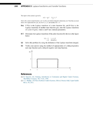
D.7. Determine the Laplace transform of the pulse function f(t) shown in the figure
below
ftðÞ ¼ 2, 1 t 5
¼ 0, elsewhere
(a) Solve this problem by using the definition of the Laplace transform integral.

(b) Verify your answer using the method of superposition of a delayed positive
unit step function and a delayed negative unit step function.

f(t)

2

0 1 5 t

References
[1] R. Saucedo, E.E. Schiring, Introduction to Continuous and Digital Control Systems,
MacMillan Company, New York, 1968.
[2] C.L. Phillips, J.M. Parr, Feedback Control Systems, fifth ed, Prentice Hall, Upper Saddle
River, NJ, 2011.