Page 298 - Dynamics and Control of Nuclear Reactors

300 APPENDIX F State variable models and transient analysis

A is an (n x n) square matrix; and xand b are (n x 1) column vectors. A matrix is
shown by an upper-case letter and a vector by a lower-case letter with an underline.
Laplace transform of a variable, z(t), is indicated by the upper-case letter, Z(s).
The element of a matrix, A, in row i and column j is denoted by a ij . If the number
of rows (m) is equal to the number of columns (n), m¼n, then A is called a square
matrix. If m 6¼ n, then A is a rectangular matrix. If most of the matrix elements are
zero, the matrix is said to be sparse. State variable matrices in nuclear reactor sim-
ulations are generally sparse, with non-zero elements clustered around the matrix
diagonal.
The A matrix for most nuclear reactors have negative diagonal elements. A pos-
itive diagonal element may exist in a model for a stable system, but instability is often
encountered for such a model. A positive diagonal element causes a suspicion
that the solution will indicate instability. If the analyst has reason to believe that
the reactor is stable, it is wise to check the correctness of a positive diagonal element.
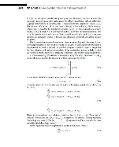
A column vector x of variables is an ordered array of scalars. A column vector x
with n elements has the dimension (n x 1) as shown in Eq. (F.4a).
2 3
x 1
x 2
6 7
6 7
6 : 7
Column Vector x ¼ 6 7 ð nx1Þ (F.4a)
:
6 7
6 7
:
4 5
x n
A row vector is defined as the transpose of a column vector.
T
½
x ¼ x 1 ,x 2 , …x n Š (F.4b)
Dynamic analysis involves the use of matrix differential equations as shown in
Eq. (F.5).
dx 1
¼ a 11 x 1 + a 12 x 2 + … + a 1n x n + f 1 + g 1
dt
dx 2
¼ a 21 x 1 + a 22 x 2 + … + a 2n x n + f 2 + g 2
dt
(F.5)
…
…
…
dx n
¼ a n1 x 1 + a n2 x 2 + … + a nn x n + f n + g n
dt
2
There are n equations in n solution variables, {x i ,i¼1, 2, …,n}. There are n
constant coefficients. The {f i , i¼1, 2, …,n} represent the external forcing functions
(including zero values). The {g i , i¼1, 2, …,n} represent nonlinear terms in the state
variables (including zero values).
These equations may be expressed in matrix notation as follows.
dx
¼ Ax + f + g (F.6)
dt