Page 297 - Dynamics and Control of Nuclear Reactors

APPENDIX

State variable models and

transient analysis F

F.1 Introduction

Models of real-world systems often require large sets of coupled differential equations to
represent all of the interconnected processes. Models involving hundreds of equations
are not uncommon. This naturally leads to the use of vector-matrix notation and to the
formulation of computer solution software packages that accept matrix formulations of
system models. These packages can accept models with any number of system equations
(up to some maximum dictated by computer capability) and generate solutions. These
simulation software packages include MATLAB (see Appendix G), MAPLE, MATH-
EMATICA, MODELICA and others. Vector-matrix formulations and matrix-oriented
solution techniques are important in dynamic modeling and simulation. The state var-
iable representation of systems (both linear and nonlinear) is described in this appendix
with emphasis on linear system models. The state variable representation was first used
by Kalman in describing the general theory of control systems [1, 2].
Both time-domain analysis of multi-input multi-output (MIMO) linear time-
invariant systems and their analysis in the Laplace domain are described in this
Appendix.

F.2 State variable models
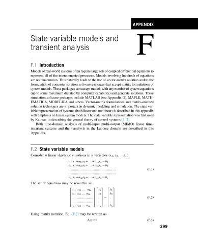
Consider n linear algebraic equations in n variables (x 1 ,x 2 , …x n ).

a 11 x 1 + a 12 x 2 + … + a 1n x n ¼ b 1
a 21 x 1 + a 22 x 2 + … + a 2n x n ¼ b 2
(F.1)
:……………………………………
:……………………………………
a n1 x 1 + a n2 x 2 + … + a nn x n ¼ b n
The set of equations may be rewritten as
2 32 3 2 3
a 11 a 12 … a 1n x 1 b 1
a 21 a 22 … a 2n 7 x 2 7
6 6 7 6 7
6 76 6 b 2 7
: ¼ : (F.2)
6 76 7 6 7
::………………
6 76 7 6 7
: :
4 54 5 4 5
::………………
a n1 a n2 … a nn x n b n
Using matrix notation, Eq. (F.2) may be written as
Ax ¼ b (F.3)
299