Page 106 - Dynamics of Mechanical Systems

0593_C04*_fm Page 87 Monday, May 6, 2002 2:06 PM

Kinematics of a Rigid Body 87

B
n 2
X
n
1
R
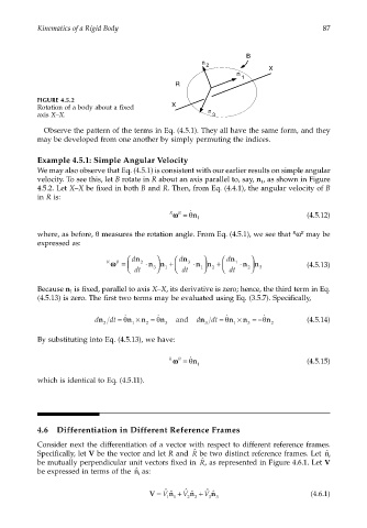
FIGURE 4.5.2
Rotation of a body about a fixed X n
axis X–X. 3
Observe the pattern of the terms in Eq. (4.5.1). They all have the same form, and they
may be developed from one another by simply permuting the indices.

Example 4.5.1: Simple Angular Velocity
We may also observe that Eq. (4.5.1) is consistent with our earlier results on simple angular
velocity. To see this, let B rotate in R about an axis parallel to, say, n , as shown in Figure
1
4.5.2. Let X–X be fixed in both B and R. Then, from Eq. (4.4.1), the angular velocity of B
in R is:
˙
B
R ωω= θn 1 (4.5.12)
where, as before, θ measures the rotation angle. From Eq. (4.5.1), we see that ω may be
B
R
expressed as:
 dn   dn   dn 



R B 2 3 1
ωω=  ⋅nn +  ⋅nn +  ⋅nn (4.5.13)
 dt 3  1  dt 1  2  dt 2  3
Because n is fixed, parallel to axis X–X, its derivative is zero; hence, the third term in Eq.
1
(4.5.13) is zero. The first two terms may be evaluated using Eq. (3.5.7). Specifically,
dn dt = θ ˙ n × n = θ ˙ n and dn dt = θ ˙ n × n = −θ ˙ n (4.5.14)
2 1 2 3 3 1 3 2

By substituting into Eq. (4.5.13), we have:

R B ˙
ωω= θn (4.5.15)
1
which is identical to Eq. (4.5.11).

4.6 Differentiation in Different Reference Frames
Consider next the differentiation of a vector with respect to different reference frames.
ˆ
Specifically, let V be the vector and let R and be two distinct reference frames. Let ˆ n i
R
ˆ
be mutually perpendicular unit vectors fixed in , as represented in Figure 4.6.1. Let V
R
ˆ n
be expressed in terms of the as:
i
ˆ
ˆ
ˆ
V = V ˆ n + V ˆ n + V n ˆ (4.6.1)
1 1 2 2 3 3