Page 111 - Dynamics of Mechanical Systems

0593_C04*_fm Page 92 Monday, May 6, 2002 2:06 PM

92 Dynamics of Mechanical Systems

ˆ
ˆ
i N i N i n i n i
N
1
2

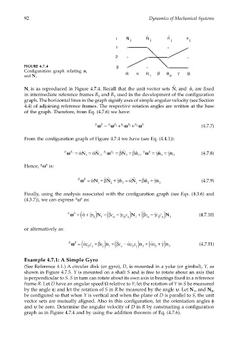
FIGURE 4.7.4 3
Configuration graph relating n i R α R β R γ B
and N i . 1 2
ˆ
N is as reproduced in Figure 4.7.4. Recall that the unit vector sets N and ˆ n are fixed
i i i
in intermediate reference frames R and R used in the development of the configuration
1 2
graph. The horizontal lines in the graph signify axes of simple angular velocity (see Section
4.4) of adjoining reference frames. The respective rotation angles are written at the base
of the graph. Therefore, from Eq. (4.7.6) we have:

B
R ωω = R ωω + R 1 ωω + R 2 ωω B (4.7.7)
R 1
R 2
From the configuration graph of Figure 4.7.4 we have (see Eq. (4.4.1)):

˙
˙ ˆ
R ωω = ˙ αN 1 = ˙ ˆ 1 , R 1 ωω R 2 = βN 2 = ˆ ,βn 2 R ωω = ˙ ˆ γn 3 = ˙ γn 3 (4.7.8)
B
αN
R 1
Hence, ω is:
B
R
R B ˙ ˆ ˙
ωω= ˙ αN + βN + ˙ ˆ γn = ˙ ˆ + ˆ + ˙ γn (4.7.9)
αN
βn
1 2 3 1 2 3
Finally, using the analysis associated with the configuration graph (see Eqs. (4.3.6) and
(4.3.7)), we can express ω as:
B
R
ωω= ( αγ s ) N 1 + β c − ˙ γ c s N 2 + β s − ˙ γ c c N 3 (4.7.10)
+ ˙
˙
R B ( ˙ ) ( ˙ )
β α
α
α
β α
β
or alternatively as:
ωω= ˙ α cc + β s n 1 + β c − ˙ α c s n 2 +( α ˙ s + ) γ n 3 (4.7.11)
R B ( ˙ ) ( ˙ )
˙
β γ
β γ
γ
γ
β
Example 4.7.1: A Simple Gyro
(See Reference 4.1.) A circular disk (or gyro), D, is mounted in a yoke (or gimbal), Y, as
shown in Figure 4.7.5. Y is mounted on a shaft S and is free to rotate about an axis that
is perpendicular to S. S in turn can rotate about its own axis in bearings fixed in a reference
frame R. Let D have an angular speed Ω relative to Y; let the rotation of Y in S be measured
by the angle φ; and let the rotation of S in R be measured by the angle ψ. Let N and N
Yi Ri
be configured so that when Y is vertical and when the plane of D is parallel to S, the unit
vector sets are mutually aligned. Also in this configuration, let the orientation angles φ
and ψ be zero. Determine the angular velocity of D in R by constructing a configuration
graph as in Figure 4.7.4 and by using the addition theorem of Eq. (4.7.6).