Page 110 - Dynamics of Mechanical Systems

0593_C04*_fm Page 91 Monday, May 6, 2002 2:06 PM

Kinematics of a Rigid Body 91

Hence, by substituting into Eq. (4.7.1) we have:

R B = R ˆ B + R R ˆ
ωω × V ωω × V ωω × V
or
( R ωω − R ˆ ωω − R ωω R ˆ ) × V = 0 (4.7.3)
B
B

Because V is arbitrary, we thus have:

ωω − ωω − ωω = 0
R B R ˆ B R R ˆ
or

ωω = ωω + ωω (4.7.4)
R B R ˆ B R R ˆ
Equation (4.7.4) is an expression of the addition theorem for angular velocity. Because
body B may itself be considered as a reference frame, Eq. (4.7.4) may be rewritten in the
form:

R 0 ωω R 2 = R 0 ωω + R 1 ωω R 2 (4.7.5)
R 1
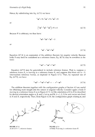
Equation (4.7.5) may be generalized to include reference frames. That is, suppose a
reference frame R is moving in a reference frame R and suppose that there are (n –1)
n
0
intermediate reference frames, as depicted in Figure 4.7.2. Then, by repeated use of
Eq. (4.7.5), we have:
R 1
R 0 ωω R n = R 0 ωω + R 1 ωω + ... + R n 1− ωω R n (4.7.6)
R 2
The addition theorem together with the configuration graphs of Section 4.3 are useful
for obtaining more insight into the nature of angular velocity. Consider again a body B
moving in a reference frame R as in Figure 4.7.3. Let the orientation of B in R be described
by dextral orientation angles α, β, and γ. Let n and N (i = 1, 2, 3) be unit vector sets fixed
i
i
in B and R, respectively. Then, from Figure 4.3.8, the configuration graph relating n and
i
R n B
n
3
R n-1 n 2
R N 3
2 n
1
R
1 R
R 0
N
2
N 1
FIGURE 4.7.2 FIGURE 4.7.3
A set of n + 1 reference frames. A body B moving in a reference frame R.