Page 101 - Dynamics of Mechanical Systems

0593_C04*_fm Page 82 Monday, May 6, 2002 2:06 PM

82 Dynamics of Mechanical Systems

n
3 n
2

N
3 n
1
R
B
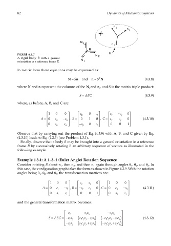
FIGURE 4.3.7
N 2
A rigid body B with a general
orientation in a reference frame R. N 1
In matrix form these equations may be expressed as:

n
N = S and n = S T N (4.3.8)
where N and n represent the columns of the N and n , and S is the matrix triple product:
i
i
S = ABC (4.3.9)

where, as before, A, B, and C are:

1 0 0   c β 0 s  c  γ s − γ  0
β
     
s
A = 0 c α s − α  , B =  0 1 0 , C =  γ c γ 0  (4.3.10)


 0 s α c     s − β 0 c β     0 0  1 
α
Observe that by carrying out the product of Eq. (4.3.9) with A, B, and C given by Eq.
(4.3.10) leads to Eq. (4.2.3) (see Problem 4.3.1).
Finally, observe that a body B may be brought into a general orientation in a reference
frame R by successively rotating B an arbitrary sequence of vectors as illustrated in the
following example.

Example 4.3.1: A 1–3–1 (Euler Angle) Rotation Sequence
Consider rotating B about n , then n , and then n again through angles θ , θ , and θ . In
1
1
3
3
1
2
this case, the configuration graph takes the form as shown in Figure 4.3.9. With the rotation
angles being θ , θ , and θ , the transformation matrices are:
3
1
2
1 0 0   c 2 s 2  0 1 0 0 
     
A = 0 c 1 s − 1  , B =− s 2 c 2 0 , C = 0 c 3 s − 3  (4.3.11)




 0 s 1 c     0 0  1   0 s 3 c  
1
3
and the general transformation matrix becomes:
 c 2 s c − s s 
2 3
2 3

S = ABC = − cs ( 1 2 3 s s ) ( − c c c − s c )   (4.3.12)
c c c −

12
1 3
1 2 3
1 3
 − s c c + c s ) ( − s c s + cc ) 
 ss ( 1 2 3 1 3 1 2 3 1 3 
12