Page 100 - Dynamics of Mechanical Systems

0593_C04*_fm Page 81 Monday, May 6, 2002 2:06 PM

Kinematics of a Rigid Body 81

ˆ
ˆ
N i N i n i
N
î 3
N
3
1
ˆ
N
α 2 2
α 3
N
2 β
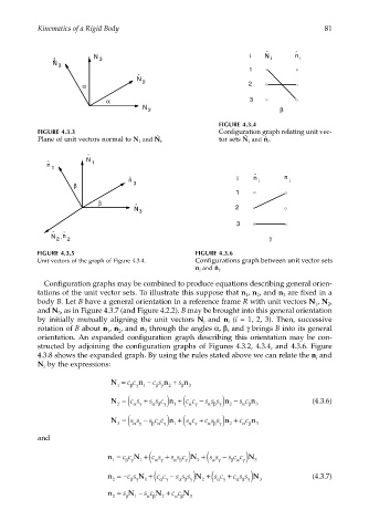
FIGURE 4.3.4
FIGURE 4.3.3 Configuration graph relating unit vec-
ˆ
ˆ
Plane of unit vectors normal to N 1 and N i . tor sets N 1 and ˆ n i .
ˆ
N
ˆ 1
n
1
ˆ
n ˆ i n i n i
β 3
1
β
ˆ
N 2
3
3
ˆ n ˆ
N , γ
2 2
FIGURE 4.3.5 FIGURE 4.3.6
Unit vectors of the graph of Figure 4.3.4. Configurations graph between unit vector sets
n i and ˆ n i .
Configuration graphs may be combined to produce equations describing general orien-
tations of the unit vector sets. To illustrate this suppose that n , n , and n are fixed in a
1
2
3
body B. Let B have a general orientation in a reference frame R with unit vectors N , N ,
1
2
and N , as in Figure 4.3.7 (and Figure 4.2.2). B may be brought into this general orientation
3
by initially mutually aligning the unit vectors N and n (i = 1, 2, 3). Then, successive
i
i
rotation of B about n , n , and n through the angles α, β, and γ brings B into its general
2
3
1
orientation. An expanded configuration graph describing this orientation may be con-
structed by adjoining the configuration graphs of Figures 4.3.2, 4.3.4, and 4.3.6. Figure
4.3.8 shows the expanded graph. By using the rules stated above we can relate the n and
i
N by the expressions:
i
N = cc n − c s n + s n
1 β γ 1 β γ 2 β 3
+
N = ( cs + s s c n ) ( c c − s s s n ) − s c n (4.3.6)
2 αγ α β γ 1 α γ α β γ 2 α β 3
+
N = ( ss − s c c n ) ( s c + c s s n ) + cc n
3 αγ β αγ 1 αγ α β γ 2 α β 3
and
N ) N )
+
n = cc N +( c s + s s c 2 ( s s − s c c
1 β γ 1 α γ α β γ α γ β αγ 3
N ) N )
+
n =−cs N +( c c − s s s 2 ( s c + c s s (4.3.7)
2 β γ 1 α γ α β γ α γ α β γ 3
n = s N − s c N + c c N
3 β 1 α β 2 α β 3