Page 102 - Dynamics of Mechanical Systems

0593_C04*_fm Page 83 Monday, May 6, 2002 2:06 PM

Kinematics of a Rigid Body 83

ˆ
ˆ
ˆ
ˆ
N
N
i N N n n i N i N i n i n i
i i i i
1 1
2 2
3 3
α β γ θ 1 θ 2 θ 3
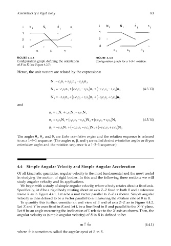
FIGURE 4.3.8 FIGURE 4.3.9
Configuration graph defining the orientation Configuration graph for a 1–3–1 rotation.
of B in R (see Figure 4.3.7).
Hence, the unit vectors are related by the expressions:

N = c n + s c n − s s n
1 2 1 2 3 2 2 3 3
n ) 2 ( n )
N =−cs n +(c c c − s s +−c c c − s c (4.3.13)
2 1 2 1 12 3 1 3 12 3 1 3 3
+−s c s
N =−ss n +(s c c + c s n ) 2 ( + cc n )
3 1 2 1 12 3 1 3 12 3 1 3 3
and
n = c 2 N + c s N − s s N 3
1 2
1 2
1
2
1
+
n = sc N +(c c c − s s N ) 2 (s c c + c s N ) 3 (4.3.14)
12 3
1 3
2
2 3
1 3
12 3
1
n =−s s N + − ( cc s − s c N ) 2 ( 12 3 + cc N ) 3
+−s c s
1
2 3
3
1 3
12 3
1 3
The angles θ , θ , and θ are Euler orientation angles and the rotation sequence is referred
1
3
2
to as a 1–3–1 sequence. (The angles α, β, and γ are called dextral orientation angles or Bryan
orientation angles and the rotation sequence is a 1–2–3 sequence.)
4.4 Simple Angular Velocity and Simple Angular Acceleration
Of all kinematic quantities, angular velocity is the most fundamental and the most useful
in studying the motion of rigid bodies. In this and the following three sections we will
study angular velocity and its applications.
We begin with a study of simple angular velocity, where a body rotates about a fixed axis.
Specifically, let B be a rigid body rotating about an axis Z–Z fixed in both B and a reference
frame R as in Figure 4.4.1. Let n be a unit vector parallel to Z–Z as shown. Simple angular
velocity is then defined to be a vector parallel to n measuring the rotation rate of B in R.
To quantify this further, consider an end view of B and of axis Z–Z as in Figure 4.4.2.
Let X and Y be axes fixed in R and let L be a line fixed in B and parallel to the X–Y plane.
Let θ be an angle measuring the inclination of L relative to the X-axis as shown. Then, the
angular velocity ω (simple angular velocity) of B in R is defined to be:
˙
D
ωω = θn (4.4.1)
θ
˙
where is sometimes called the angular speed of B in R.