Page 156 - Dynamics of Mechanical Systems

0593_C05_fm Page 137 Monday, May 6, 2002 2:15 PM

Planar Motion of Rigid Bodies — Methods of Analysis 137

Y
φ θ 3
2
β
2 β
θ 3
φ 2
1
φ
3
θ 1 β 1
X

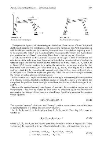
FIGURE 5.5.2 FIGURE 5.5.3
Absolute orientation angles. Relative orientation angles.

The system of Figure 5.5.1 has one degree of freedom: The rotations of bars OP(B ) and
1
RQ(B ) each require two coordinates, and the general motion of bar PQ(B ) requires an
2
3
additional three coordinates for a total of five coordinates. Nevertheless, requiring joint P
to be connected to both B and B and joint Q to be connected to both B and B produces
2
2
1
3
four position (or coordinate) constraints. Thus, there is but one degree of freedom.
A task encountered in the kinematic analyses of linkages is that of describing the
orientation of the individual bars. One method is to define the orientations of the bars in
terms of angles that the bars make with the horizontal (or X-axis) such as θ , θ , and θ as
3
1
2
in Figure 5.5.2. Another method is to define the orientation in terms of angles that the
bars make with the vertical (or Y-axis) such as φ , φ , and φ as in Figure 5.5.2. A third
3
1
2
method is to define the orientations in terms of angles that the bars make with each other,
as in Figure 5.5.3. The latter angles are generally called relative orientation angles whereas
the former are called absolute orientation angles.
Relative orientation angles are usually more meaningful in describing the configuration
of a physical system. Absolute orientation angles are usually easier to work with in the
analysis of the problem. In our example, we will use the first set of absolute angles θ , θ ,
2
1
and θ .
3
Because the system has only one degree of freedom, the orientation angles are not
independent. They may be related to each other by constraint equations obtained by
considering the linkage of four bars as a closed loop: Specifically, consider the position
vector equation:
+
+
+
OP PQ QR RO = 0 (5.5.1)
This equation locates O relative to itself through position vectors taken around the loop
of the mechanism. It is called the loop closure equation.
Let , , , and be the lengths of bars B , B , B , and B . Then, Eq. (5.5.1) may be
4
1
2
3
3
4
2
1
written as:
l λλ + l λλ + l λλ + l λλ = 0 (5.5.2)
4
2
3
3
4
1 1
2
where λλ λλ , λλ λλ , λλ λλ , and λλ λλ are unit vectors parallel to the rods as shown in Figure 5.5.4. These
2
3
4
1
vectors may be expressed in terms of horizontal and vertical unit vectors n and n as:
y
x
λλ = cosθ n + sinθ n , λλ = cosθ n + sinθ n
1 1 x 1 y 2 2 x 2 y (5.5.3)
λλ = cosθ n − sinθ n , λλ = −n
3 3 x 3 4 4 x