Page 157 - Dynamics of Mechanical Systems

0593_C05_fm Page 138 Monday, May 6, 2002 2:15 PM

138 Dynamics of Mechanical Systems

Y B 2
λ θ 3
n y 2

B θ B 3
1 2
λ
1
λ
3
O θ 1 λ 4 R X
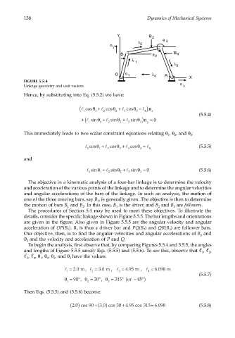
FIGURE 5.5.4
Linkage geometry and unit vectors. n x
Hence, by substituting into Eq. (5.5.2) we have:

1 (
l cosθ + l cosθ + l cosθ − )n x
l
1
2
2
3
3
4
(5.5.4)
1 (
+ l sinθ + l sinθ + l sinθ )n y = 0
2
3
1
3
2
This immediately leads to two scalar constraint equations relating θ , θ , and θ :
1 2 3
l cosθ + l cosθ + l cosθ = l (5.5.5)
1 1 2 2 3 3 4
and
l sinθ + l sinθ + l sinθ = 0 (5.5.6)
2
3
1
2
3
1
The objective in a kinematic analysis of a four-bar linkage is to determine the velocity
and acceleration of the various points of the linkage and to determine the angular velocities
and angular accelerations of the bars of the linkage. In such an analysis, the motion of
one of the three moving bars, say B , is generally given. The objective is then to determine
1
the motion of bars B and B . In this case, B is the driver, and B and B are followers.
1 2 1 2 3
The procedures of Section 5.4 may be used to meet these objectives. To illustrate the
details, consider the specific linkage shown in Figure 5.5.5. The bar lengths and orientations
are given in the figure. Also given in Figure 5.5.5 are the angular velocity and angular
acceleration of OP(B ). B is thus a driver bar and PQ(B ) and QR(B ) are follower bars.
1 1 2 3
Our objective, then, is to find the angular velocities and angular accelerations of B and
2
B and the velocity and acceleration of P and Q.
3
To begin the analysis, first observe that, by comparing Figures 5.5.4 and 5.5.5, the angles
and lengths of Figure 5.5.5 satisfy Eqs. (5.5.5) and (5.5.6). To see this, observe that , ,
1 2
, , θ , θ , θ , and θ have the values:
3 4 1 2 3 4
l = 20 m, l = 30 m , l = 495 m , l = 6 098 m
.
.
.
.
1 2 3 4 (5.5.7)
θ = 90°, θ = 30°, θ = 315° ( or – 45 °)
1 2 3
Then Eqs. (5.5.5) and (5.5.6) become:
. ( )
+
=
.
3 0 cos
.
2 0 cos 90 +( ) 30 4 95 cos 315 6 098 (5.5.8)
.