Page 38 - Earth's Climate Past and Future

14 PART I • Framework of Climate Science

The main difference now is that the climate forcing
Fast
(the intensity of the flame from the Bunsen burner) is response
constantly changing, rather than holding at a single con-
stant equilibrium value (as in Figure 1-6) or switching
between two equilibrium values in an alternating Slow
sequence (as in Figures 1-7C and D). The continuous response
changes in heating act as a “moving target.” The climate
system response (the water temperature) keeps chasing
this moving target but can never catch up to it because
the water temperature cannot respond quickly enough.
As was the case for the on-off changes shown in
Figures 1-7C and D, the frequency with which these
smooth cycles of forcing occur has a direct effect on the Forcing
amplitude of the responses. This effect is apparent turned on
in the differences between the cases shown in Figures
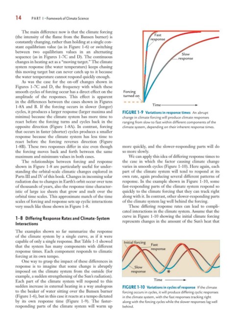
1-8A and B. If the forcing occurs in slower (longer) Time
cycles, it produces a larger response (larger maxima and FIGURE 1-9 Variations in response times An abrupt
minima) because the climate system has more time to change in climate forcing will produce climate responses
react before the forcing turns and cycles back in the ranging from slow to fast within different components of the
opposite direction (Figure 1-8A). In contrast, forcing climate system, depending on their inherent response times.
that occurs in faster (shorter) cycles produces a smaller
response because the climate system has less time to
react before the forcing reverses direction (Figure
1-8B). These two responses differ in size even though more quickly, and the slower-responding parts will do
the forcing moves back and forth between the same so more slowly.
maximum and minimum values in both cases. We can apply this idea of differing response times to
The relationships between forcing and response the case in which the factor causing climate change
shown in Figure 1-8 are particularly useful for under- varies in smooth cycles (Figure 1-10). Here again, each
standing the orbital-scale climatic changes explored in part of the climate system will tend to respond at its
Parts III and IV of this book. Changes in incoming solar own rate, again producing several different patterns of
radiation due to changes in Earth’s orbit occur over tens response. In the example shown in Figure 1-10, some
of thousands of years, also the response time character- fast-responding parts of the climate system respond so
istic of large ice sheets that grow and melt over the quickly to the climate forcing that they can track right
orbital time scales. This approximate match of the time along with it. In contrast, other slower-responding parts
scales of forcing and response sets up cyclic interactions of the climate system lag well behind the forcing.
very much like those shown in Figure 1-8. These differing response rates can lead to compli-
cated interactions in the climate system. Assume that the
curve in Figure 1-10 showing the initial climate forcing
1-8 Differing Response Rates and Climate-System
Interactions represents changes in the amount of the Sun’s heat that
The examples shown so far summarize the response
of the climate system by a single curve, as if it were
capable of only a single response. But Table 1-1 showed Initial forcing
that the system has many components with different Fast
response times. Each component responds to climatic response
forcing at its own tempo.
One way to grasp the impact of these differences in
response is to imagine that some change is abruptly Slow
imposed on the climate system from the outside (for response
example, a sudden strengthening of the Sun’s radiation).
Each part of the climate system will respond to this Time
sudden increase in external heating in a way analogous FIGURE 1-10 Variations in cycles of response If the climate
to the beaker of water sitting over the Bunsen burner forcing occurs in cycles, it will produce differing cyclic responses
(Figure 1-6), but in this case it reacts at a tempo dictated in the climate system, with the fast responses tracking right
by its own response time (Figure 1-9). The faster- along with the forcing cycles while the slower responses lag well
responding parts of the climate system will warm up behind.