Page 51 - Electrical Safety of Low Voltage Systems

34 Chapter Three

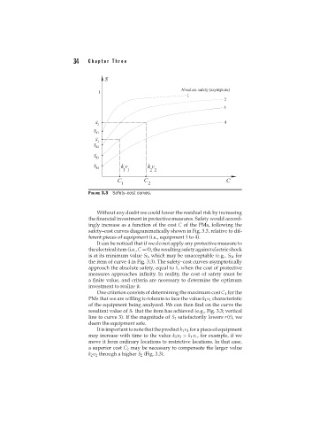
FIGURE 3.3 Safety–cost curves.

Without any doubt we could lower the residual risk by increasing
the financial investment in protective measures. Safety would accord-
ingly increase as a function of the cost C of the PMs, following the
safety–cost curves diagrammatically shown in Fig. 3.3, relative to dif-
ferent pieces of equipment (i.e., equipment 1 to 4).
It can be noticed that if we do not apply any protective measure to
theelectricalitem(i.e.,C =0),theresultingsafetyagainstelectricshock
is at its minimum value S 0 , which may be unacceptable (e.g., S 04 for
the item of curve 4 in Fig. 3.3). The safety–cost curves asymptotically
approach the absolute safety, equal to 1, when the cost of protective
measures approaches infinity. In reality, the cost of safety must be
a finite value, and criteria are necessary to determine the optimum
investment to realize it.
One criterion consists of determining the maximum cost C 1 for the
PMs that we are willing to tolerate to face the value k 1 v 1 characteristic
of the equipment being analyzed. We can then find on the curve the
resultant value of S 1 that the item has achieved (e.g., Fig. 3.3; vertical
line to curve 3). If the magnitude of S 1 satisfactorily lowers r(t), we
deem the equipment safe.
Itisimportanttonotethattheproductk 1 v 1 forapieceofequipment
may increase with time to the value k 2 v 2 > k 1 v 1 , for example, if we
move it from ordinary locations to restrictive locations. In that case,
a superior cost C 2 may be necessary to compensate the larger value
k 2 v 2 through a higher S 2 (Fig. 3.3).