Page 52 - Electrical Safety of Low Voltage Systems

Mathematical Principles of Electrical Safety 35

Alternatively, one might establish the desired level of safety S 1
and accordingly determine the relative cost C 1 . If the magnitude of
the cost C 1 falls within the allocated budget, we achieve the desired
safety.
With the above methodologies, results may be unacceptable to the
designer: in the first case, S 1 may be too low and one must increase
the cost; in the latter case, the cost C 1 may exceed the available bud-
get, which forces the designer to lower the desired value S 1 . In other
cases, it can be realized that small increases in cost can remarkably
raise safety and, vice versa, minimum decreases in safety may allow
substantial reductions in costs.
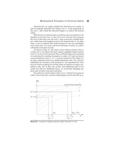
As shown in Fig. 3.3, the safety curves almost saturate when a
certain cost is exceeded and show almost negligible improvements
even if C is very much increased. Thus, a different approach consisting
of evaluating the resulting increments in safety S i from successive
unit increments in cost (i.e., C = 1) can be carried out. The values S i
are then compared with an acceptable minimum value S 0 , which is
established as a function of the product kv. S 0 represents the value
beyond which investing in lowering safety is deemed no longer cost-
effective (Fig. 3.4). In this case, in fact, each additional unit of cost
yields less and less additional safety, or, conversely, obtaining one
more unit of safety costs more and more.
The optimum cost for safety in Fig. 3.4 is C 1 . Should kv increase, in
order to lower the risk, we must accept higher costs for the PMs (e.g.,

FIGURE 3.4 Increment in safety caused by unitary increment of cost.