Page 129 - Electrical Properties of Materials

The Feynman model 111

E

E +2A
1

E
1

E –2A
1
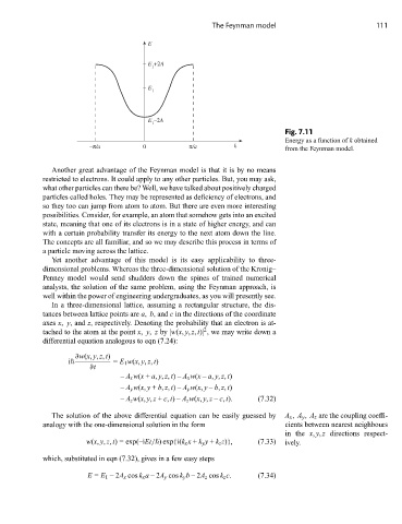
Fig. 7.11
Energy as a function of k obtained
–π/a 0 π/a k from the Feynman model.

Another great advantage of the Feynman model is that it is by no means
restricted to electrons. It could apply to any other particles. But, you may ask,
what other particles can there be? Well, we have talked about positively charged
particles called holes. They may be represented as deficiency of electrons, and
so they too can jump from atom to atom. But there are even more interesting
possibilities. Consider, for example, an atom that somehow gets into an excited
state, meaning that one of its electrons is in a state of higher energy, and can
with a certain probability transfer its energy to the next atom down the line.
The concepts are all familiar, and so we may describe this process in terms of
a particle moving across the lattice.
Yet another advantage of this model is its easy applicability to three-
dimensional problems. Whereas the three-dimensional solution of the Kronig–
Penney model would send shudders down the spines of trained numerical
analysts, the solution of the same problem, using the Feynman approach, is
well within the power of engineering undergraduates, as you will presently see.
In a three-dimensional lattice, assuming a rectangular structure, the dis-
tances between lattice points are a, b, and c in the directions of the coordinate
axes x, y, and z, respectively. Denoting the probability that an electron is at-
2
tached to the atom at the point x, y, z by |w(x, y, z, t)| , we may write down a
differential equation analogous to eqn (7.24):

∂w(x, y, z, t)
i = E 1 w(x, y, z, t)
∂t
– A x w(x + a, y, z, t)– A x w(x – a, y, z, t)
– A y w(x, y + b, z, t)– A y w(x, y – b, z, t)
– A z w(x, y, z + c, t)– A z w(x, y, z – c, t). (7.32)
The solution of the above differential equation can be easily guessed by A x , A y , A z are the coupling coeffi-
analogy with the one-dimensional solution in the form cients between nearest neighbours
in the x, y, z directions respect-
w(x, y, z, t)=exp(–iEt/ )exp{i(k x x + k y y + k z z)}, (7.33) ively.

which, substituted in eqn (7.32), gives in a few easy steps
E = E 1 –2A x cos k x a –2A y cos k y b –2A z cos k z c. (7.34)