Page 126 - Electrical Properties of Materials

108 The band theory of solids

The integration in eqn (7.19) can be easily performed, but we are not really
E
interested in the actual numerical values. The important thing is that V n = 0
and has opposite signs for the wave functions ψ ± .
Let us go through the argument again. If the electron waves have certain
wave numbers [satisfying eqn (7.15)], they are reflected by the lattice. For each
value of k two distinct wave functions ψ + and ψ – can be constructed, and the
corresponding potential energies turn out to be +V n and –V n .
The kinetic energies are the same for both wave functions, namely

2 2
k
E = . (7.21)
2m
E+
Thus, the total energies are
E–
2 2
k
k E ± = ± V n . (7.22)
π/a 2m
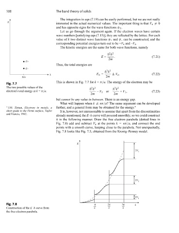
This is shown in Fig. 7.7 for k = π/a. The energy of the electron may be
Fig. 7.7
The two possible values of the k k
2 2
2 2
electron’s total energy at k = π/a. – V 1 or + V 1 , (7.23)
2m 2m
but cannot be any value in between. There is an energy gap.
What will happen when k = nπ/a? The same argument can be developed
∗ J.M. Ziman, Electrons in metals, a further, and a general form may be obtained for the energy. ∗
short guide to the Fermi surface,Taylor It is, however, not unreasonable to assume that apart from the discontinuities
and Francis, 1962.
already mentioned, the E–k curve will proceed smoothly; so we could construct
it in the following manner. Draw the free electron parabola (dotted lines in
Fig. 7.8) add and subtract V n at the points k = nπ/a, and connect the end
points with a smooth curve, keeping close to the parabola. Not unexpectedly,
Fig. 7.8 looks like Fig. 7.5, obtained from the Kronig–Penney model.

E

2V
3

2V
2

2V 1

Fig. 7.8 π 2π 3π k
Construction of the E–k curve from a a a
the free-electron parabola.