Page 134 - Electrical Properties of Materials

116 The band theory of solids

x

1 2
N 3
a 4
N 5
a–1

L

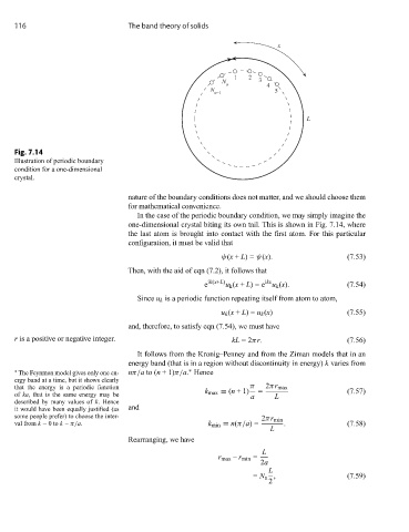
Fig. 7.14
Illustration of periodic boundary
condition for a one-dimensional
crystal.

nature of the boundary conditions does not matter, and we should choose them
for mathematical convenience.
In the case of the periodic boundary condition, we may simply imagine the
one-dimensional crystal biting its own tail. This is shown in Fig. 7.14, where
the last atom is brought into contact with the first atom. For this particular
configuration, it must be valid that

ψ(x + L)= ψ(x). (7.53)
Then, with the aid of eqn (7.2), it follows that
ik(x+L) ikx
e u k (x + L)=e u k (x). (7.54)
Since u k is a periodic function repeating itself from atom to atom,

u k (x + L)= u k (x) (7.55)
and, therefore, to satisfy eqn (7.54), we must have
r is a positive or negative integer. kL =2πr. (7.56)

It follows from the Kronig–Penney and from the Ziman models that in an
energy band (that is in a region without discontinuity in energy) k varies from
∗
∗ The Feynman model gives only one en- nπ/a to (n +1)π/a. Hence
ergy band at a time, but it shows clearly
that the energy is a periodic function π 2πr max
of ka, that is the same energy may be k max ≡ (n +1) a = L (7.57)
describedbymanyvaluesof k. Hence
it would have been equally justified (as and
some people prefer) to choose the inter-
2πr min
val from k =0 to k = π/a. k min ≡ n(π/a)= . (7.58)
L
Rearranging, we have
L
r max – r min =
2a
L
= N a , (7.59)
2