Page 379 - Electrical Properties of Materials

Nonlinear Fabry–Perot cavities 361

I (a) I (b)
t t

B
C C
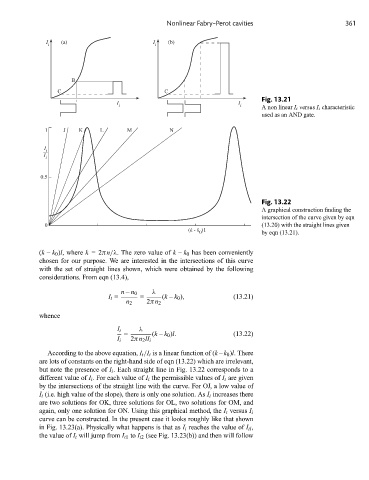
Fig. 13.21
I I
i i A non linear I t versus I i characteristic
used as an AND gate.
1 J K L M N

I t
I
i

0.5

Fig. 13.22
A graphical construction finding the
intersection of the curve given by eqn
0 (13.20) with the straight lines given
(k - k )1
0 by eqn (13.21).

(k – k 0 )l, where k =2πn/λ. The zero value of k – k 0 has been conveniently
chosen for our purpose. We are interested in the intersections of this curve
with the set of straight lines shown, which were obtained by the following
considerations. From eqn (13.4),

n – n 0 λ
I t = = (k – k 0 ), (13.21)
n 2 2πn 2
whence

I t λ
= (k – k 0 )l. (13.22)
I i 2πn 2 lI i
According to the above equation, I t /I i is a linear function of (k – k 0 )l. There
are lots of constants on the right-hand side of eqn (13.22) which are irrelevant,
but note the presence of I i . Each straight line in Fig. 13.22 corresponds to a
different value of I i . For each value of I i the permissible values of I t are given
by the intersections of the straight line with the curve. For OJ, a low value of
I i (i.e. high value of the slope), there is only one solution. As I i increases there
are two solutions for OK, three solutions for OL, two solutions for OM, and
again, only one solution for ON. Using this graphical method, the I t versus I i
curve can be constructed. In the present case it looks roughly like that shown
in Fig. 13.23(a). Physically what happens is that as I i reaches the value of I il ,
the value of I t will jump from I t1 to I t2 (see Fig. 13.23(b)) and then will follow