Page 192 - Electromagnetics

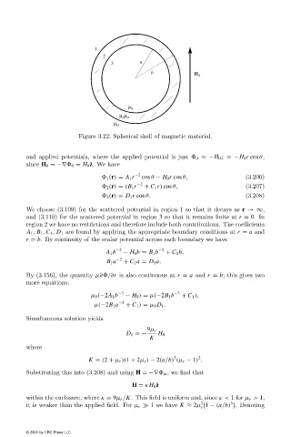
Figure 3.22: Spherical shell of magnetic material.

and applied potentials, where the applied potential is just 0 =−H 0 z =−H 0 r cos θ,
since H 0 =−∇ 0 = H 0 ˆ z. We have

1 (r) = A 1 r −2 cos θ − H 0 r cos θ, (3.206)
2 (r) = (B 1 r −2 + C 1 r) cos θ, (3.207)
3 (r) = D 1 r cos θ. (3.208)

We choose (3.109)for the scattered potential in region 1 so that it decays as r →∞,
and (3.110)for the scattered potential in region 3 so that it remains finite at r = 0.In
region 2 we have no restrictions and therefore include both contributions. The coefficients
A 1 , B 1 , C 1 , D 1 are found by applying the appropriate boundary conditions at r = a and
r = b. By continuity of the scalar potential across each boundary we have

A 1 b −2 − H 0 b = B 1 b −2 + C 1 b,
B 1 a −2 + C 1 a = D 1 a.
By (3.156), the quantity µ∂ /∂r is also continuous at r = a and r = b; this gives two
more equations:
µ 0 (−2A 1 b −3 − H 0 ) = µ(−2B 1 b −3 + C 1 ),
µ(−2B 1 a −3 + C 1 ) = µ 0 D 1 .

Simultaneous solution yields

9µ r
D 1 =− H 0
K
where
3 2
K = (2 + µ r )(1 + 2µ r ) − 2(a/b) (µ r − 1) .
Substituting this into (3.208)and using H =−∇ m , we find that
H = κ H 0 ˆ z

within the enclosure, where κ = 9µ r /K. This field is uniform and, since κ< 1 for µ r > 1,
2
3
it is weaker than the applied field. For µ r 1 we have K ≈ 2µ [1 − (a/b) ]. Denoting
r

© 2001 by CRC Press LLC