Page 196 - Electromagnetics

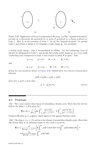
Figure 3.25: Application of Green’s reciprocation theorem. (a)The “unprimed situation”
permits us to determine the potential V P at point P produced by a charge q placed on
body 1. Here V 1 is the potential of body 1. (b)In the “primed situation” we ground

body 1 and induce a charge q by bringing a point charge q into proximity.
P
a nearby point charge. This is accomplished as follows. Let the conducting body of
interest be designated as body 1, and model the nearby point charge q P as a very small
conducting body designated as body 2 and located at point P in space. Take
q 1 = q, q 2 = 0, 1 = V 1 , 2 = V P ,
and

q = q , q = q , = 0, = V ,
P
1
1
P
2
2
giving the two situations shown in Figure 3.25. Substitution into Green’s reciprocation
theorem

q 1 + q 2 = q 1 + q 2 2
1
2
1
gives q V 1 + q V P = 0 so that

P

q =−q V P /V 1 . (3.211)
P
3.5 Problems
3.1 The z-axis carries a line charge of nonuniform density ρ l (z). Show that the electric
field in the plane z = 0 is given by

1 ∞ ρ l (z ) dz ∞ ρ l (z )z dz

E(ρ, φ) = ˆ ρρ − ˆ z .
2 3/2
4π −∞ (ρ + z ) −∞ (ρ + z )
2 3/2
2
2
Compute E when ρ l = ρ 0 sgn(z), where sgn(z) is the signum function (A.6).
3.2 The ring ρ = a, z = 0, carries a line charge of nonuniform density ρ l (φ). Show that
the electric field at an arbitrary point on the z-axis is given by
−a 2 2π 2π

E(z) = ˆ x ρ l (φ ) cos φ dφ + ˆ y ρ l (φ ) sin φ dφ +
2
2 3/2
4π (a + z ) 0 0
az 2π

+ ˆ z ρ l (φ ) dφ .

2
2 3/2
4π (a + z ) 0
© 2001 by CRC Press LLC