Page 195 - Electromagnetics

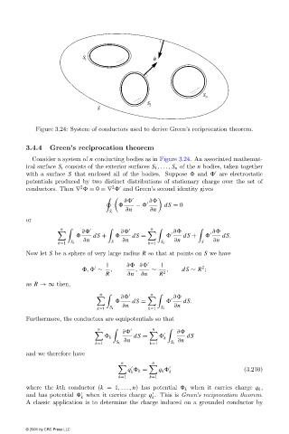
Figure 3.24: System of conductors used to derive Green’s reciprocation theorem.

3.4.4 Green’s reciprocation theorem
Consider a system of n conducting bodies as in Figure 3.24. An associated mathemat-
ical surface S t consists of the exterior surfaces S 1 ,..., S n of the n bodies, taken together

with a surface S that enclosed all of the bodies. Suppose and are electrostatic
potentials produced by two distinct distributions of stationary charge over the set of
2
2
conductors. Then ∇ = 0 =∇ and Green’s second identity gives

∂ ∂

− dS = 0
∂n ∂n
S t
or
n n

∂ ∂
∂ ∂
dS + dS = dS + dS.
∂n ∂n ∂n ∂n
k=1 S k S k=1 S k S
Now let S be a sphere of very large radius R so that at points on S we have
1 ∂ ∂ 1
2
, ∼ , , ∼ , dS ∼ R ;
R ∂n ∂n R 2
as R →∞ then,
n n

∂
∂
dS = dS.
∂n ∂n
k=1 S k k=1 S k
Furthermore, the conductors are equipotentials so that
n n

∂
∂
k dS = k dS
∂n ∂n
k=1 S k k=1 S k
and we therefore have
n n

q k = q k k (3.210)
k
k=1 k=1
where the kth conductor (k = 1,..., n)has potential k when it carries charge q k ,

and has potential when it carries charge q . This is Green’s reciprocation theorem.
k k
A classic application is to determine the charge induced on a grounded conductor by

© 2001 by CRC Press LLC